Plot diversity surfaces and their uncertainty

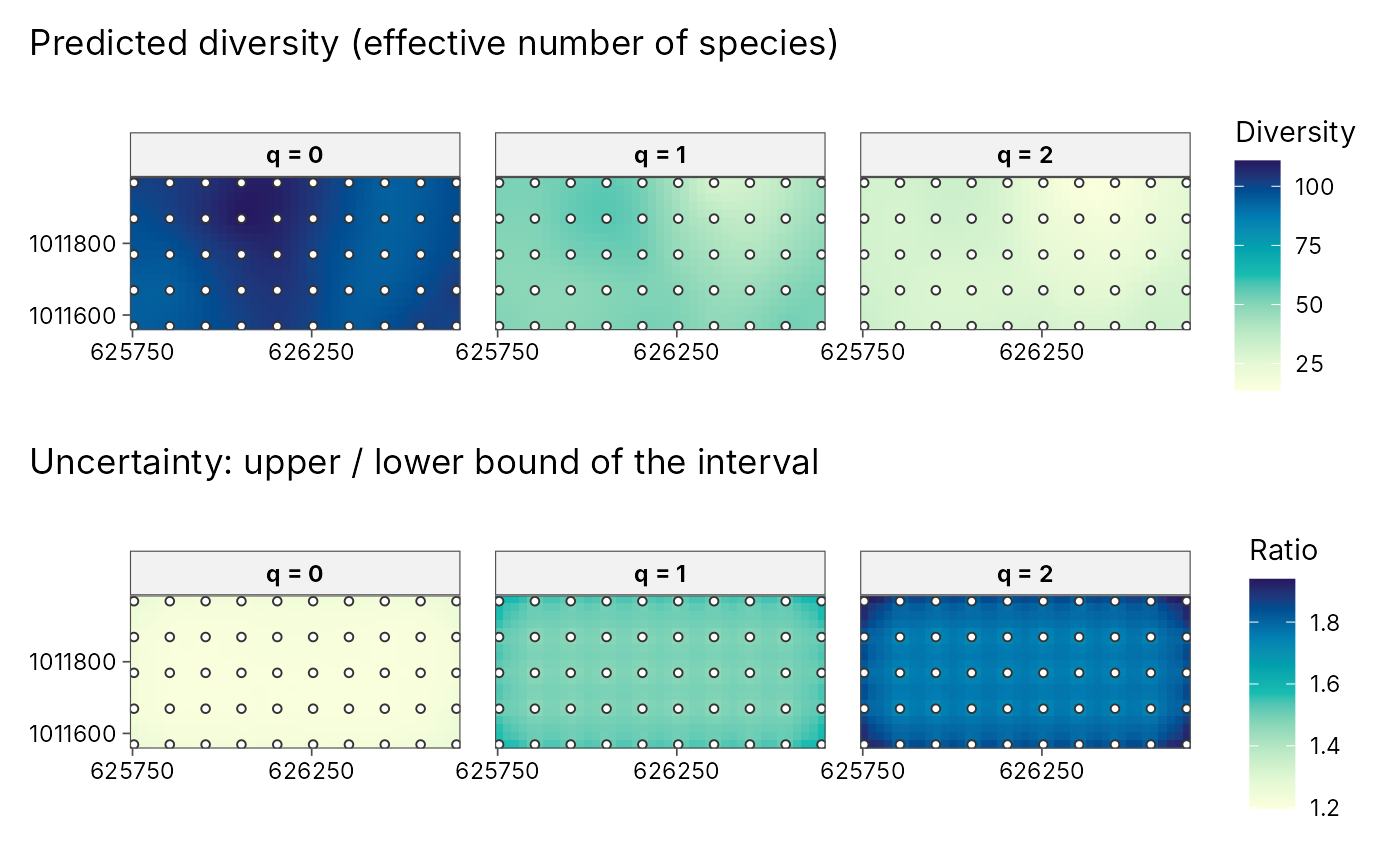
Draws the result of geo_diversity_surface(): one panel per order q (predicted diversity) and, with uncertainty = TRUE, a second row with the relative width of the prediction interval (upper / lower), so you can see where the map is well supported by data. Sampled sites are overlaid.

Usage

plot_diversity_surface(x, uncertainty = TRUE, palette = "YlGnBu", sites = TRUE)

Arguments

x

Output of geo_diversity_surface().

uncertainty

Add the uncertainty row?

palette

Sequential palette name from grDevices::hcl.pals().

sites

Overlay the sampled sites?

Value

A ggplot (or a patchwork of two when uncertainty = TRUE and patchwork is installed).

Examples

e <- new.env()
utils::data(BCI, BCI.env, package = "vegan", envir = e)
trees <- tibble::tibble(
  plot = rep(sprintf("P%02d", 1:50), ncol(e$BCI)),
  species = rep(colnames(e$BCI), each = 50),
  n = as.vector(as.matrix(e$BCI))
)
trees <- trees[trees$n > 0, ]
plots <- tibble::tibble(
  plot = sprintf("P%02d", 1:50),
  x = e$BCI.env$UTM.EW, y = e$BCI.env$UTM.NS
)
set.seed(1)
surf <- geo_diversity_surface(trees, plot, species, n,
  sites = plots, lon = x, lat = y, crs = 32617, grid = 40, nboot = 20
)
plot_diversity_surface(surf)