Case study: tree diversity across Barro Colorado Island

The 50-hectare forest dynamics plot on Barro Colorado Island, Panama, is one of the best-studied tropical forests on Earth. Every tree of at least 10 cm diameter was counted in fifty 1-hectare subplots (Condit et al. 2002; shipped with the vegan package). This case study asks where in the plot tree diversity is high or low, and how sure we can be, combining tidydiversity with tidymapr.

library(tidymapr)
library(tidydiversity)
library(dplyr)

Data

e <- new.env()
utils::data(BCI, BCI.env, package = "vegan", envir = e)

trees <- tibble::tibble(
  plot = rep(sprintf("P%02d", 1:50), ncol(e$BCI)),
  species = rep(colnames(e$BCI), each = 50),
  n = as.vector(as.matrix(e$BCI))
) |>
  filter(n > 0)

plots <- tibble::tibble(
  plot = sprintf("P%02d", 1:50),
  x = e$BCI.env$UTM.EW, y = e$BCI.env$UTM.NS,
  habitat = e$BCI.env$Habitat
)
trees
#> # A tibble: 4,539 × 3
#>    plot  species                   n
#>    <chr> <chr>                 <int>
#>  1 P10   Abarema.macradenia        1
#>  2 P28   Vachellia.melanoceras     2
#>  3 P32   Vachellia.melanoceras     1
#>  4 P34   Acalypha.diversifolia     1
#>  5 P40   Acalypha.diversifolia     1
#>  6 P28   Acalypha.macrostachya     1
#>  7 P04   Adelia.triloba            3
#>  8 P05   Adelia.triloba            1
#>  9 P09   Adelia.triloba            5
#> 10 P12   Adelia.triloba            1
#> # ℹ 4,529 more rows

Diversity per subplot

tidydiversity estimates Hill numbers of order q = 0, 1 and 2 (species richness, the exponential of Shannon entropy and inverse Simpson), standardised to the same sample coverage so that subplots can be compared.

div <- div_standardise(trees, site = plot, species = species, abundance = n, q = c(0, 1, 2), nboot = 0)
div
#> # A tibble: 150 × 9
#>    plot      q     m method        coverage diversity    se lower upper
#>    <chr> <dbl> <dbl> <chr>            <dbl>     <dbl> <dbl> <dbl> <dbl>
#>  1 P10       0  583. extrapolation    0.940     101.     NA    NA    NA
#>  2 P10       1  583. extrapolation    0.940      50.2    NA    NA    NA
#>  3 P10       2  583. extrapolation    0.940      30.1    NA    NA    NA
#>  4 P28       0  483. extrapolation    0.940      91.7    NA    NA    NA
#>  5 P28       1  483. extrapolation    0.940      41.6    NA    NA    NA
#>  6 P28       2  483. extrapolation    0.940      20.2    NA    NA    NA
#>  7 P32       0  451. rarefaction      0.940      87.5    NA    NA    NA
#>  8 P32       1  451. rarefaction      0.940      43.9    NA    NA    NA
#>  9 P32       2  451. rarefaction      0.940      23.0    NA    NA    NA
#> 10 P34       0  567. extrapolation    0.940     100.     NA    NA    NA
#> # ℹ 140 more rows

The plot and its habitats

Each 1-ha subplot drawn as a square, coloured by habitat, with its richness written on it.

squares <- sf::st_as_sf(plots, coords = c("x", "y"), crs = 32617) |>
  sf::st_buffer(50, endCapStyle = "SQUARE")
rich <- div |> filter(q == 0) |> select(plot, richness = diversity)
squares <- left_join(squares, rich, by = "plot")
squares$label <- round(squares$richness)

geo_map(title = "Barro Colorado Island 50-ha plot", caption = "Data: Condit et al. (2002), via vegan") |>
  map_polygons(squares, fill = habitat, group = "Habitat", border = "white", linewidth = 0.4) |>
  map_labels(squares, text = label, size = 2.6)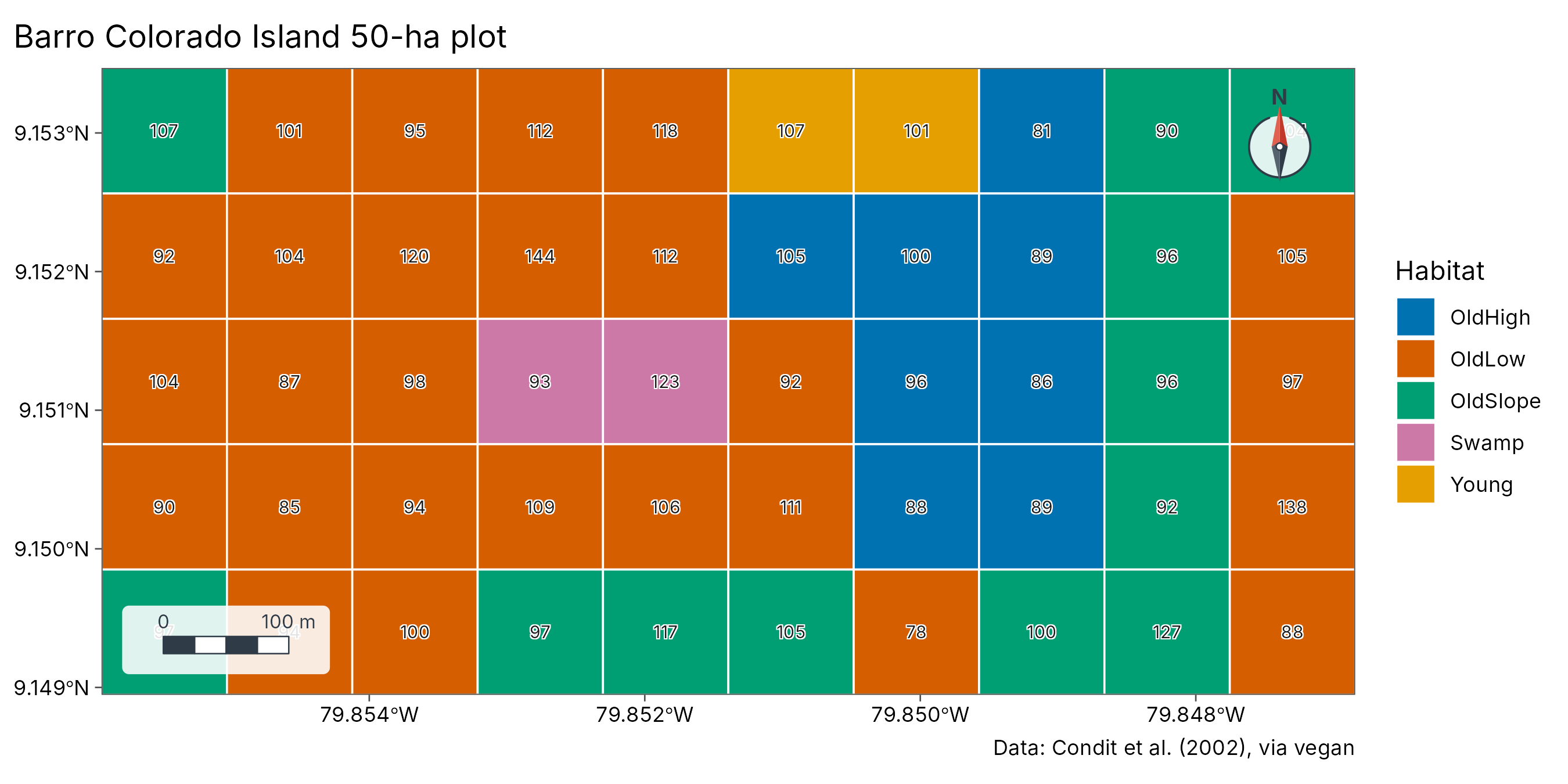

A diversity surface with its uncertainty

geo_diversity_surface() turns the subplot estimates into continuous maps by kriging on the log scale, taking each subplot’s own estimation error into account (bootstrap standard errors), and maps the width of the interval alongside.

set.seed(1)
surf <- geo_diversity_surface(trees, plot, species, n,
  sites = plots, lon = x, lat = y, crs = 32617, grid = 60, nboot = 50
)
plot_diversity_surface(surf)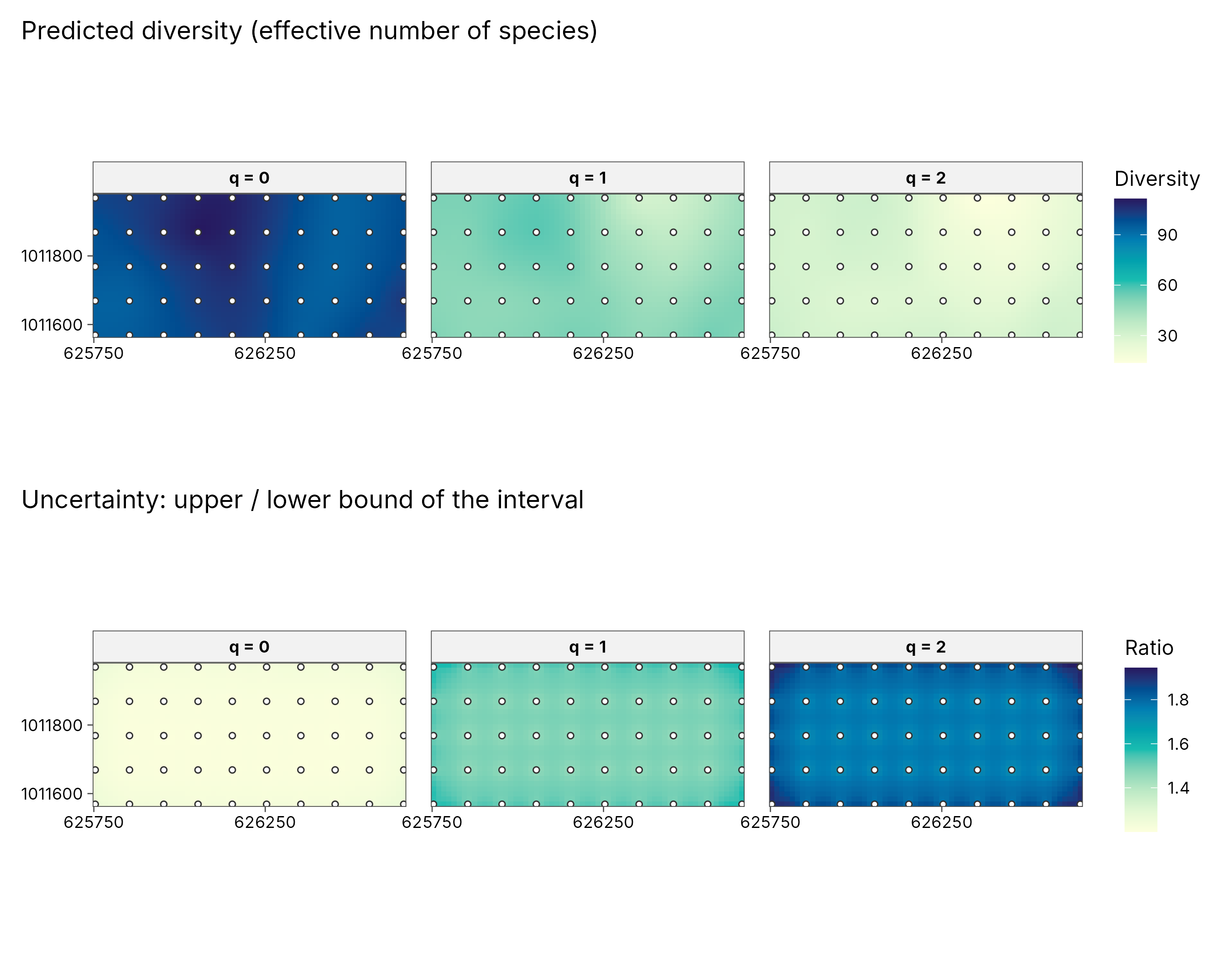

How to read the uncertainty maps. Each subplot’s diversity is an estimate, not an exact count, so every point on the surface comes with a 95% interval: the range the true value very probably lies in. The lower row maps how wide that interval is, as the upper bound divided by the lower bound. A ratio of 1.4 means the true value could be up to 40% higher than the low end of the range; a ratio of 1.8 means up to 80%. Pale areas are estimated precisely; dark areas are uncertain, so differences there should be read with caution. Uncertainty grows from q = 0 to q = 2 here because inverse Simpson depends on the few commonest species, whose share varies more from plot to plot.

Richness as a layered map

centres <- sf::st_as_sf(plots, coords = c("x", "y"), crs = 32617)
outline <- sf::st_as_sf(sf::st_union(squares))
geo_map(title = "Tree species richness (q = 0), coverage-standardised") |>
  map_raster(surf[["q0"]], name = "Species", palette = "YlGnBu") |>
  map_polygons(outline, fill = NA, preset = "study_area", label = "50-ha plot") |>
  map_points(centres, preset = "sample_site", label = "Subplot centre", size = 1.4)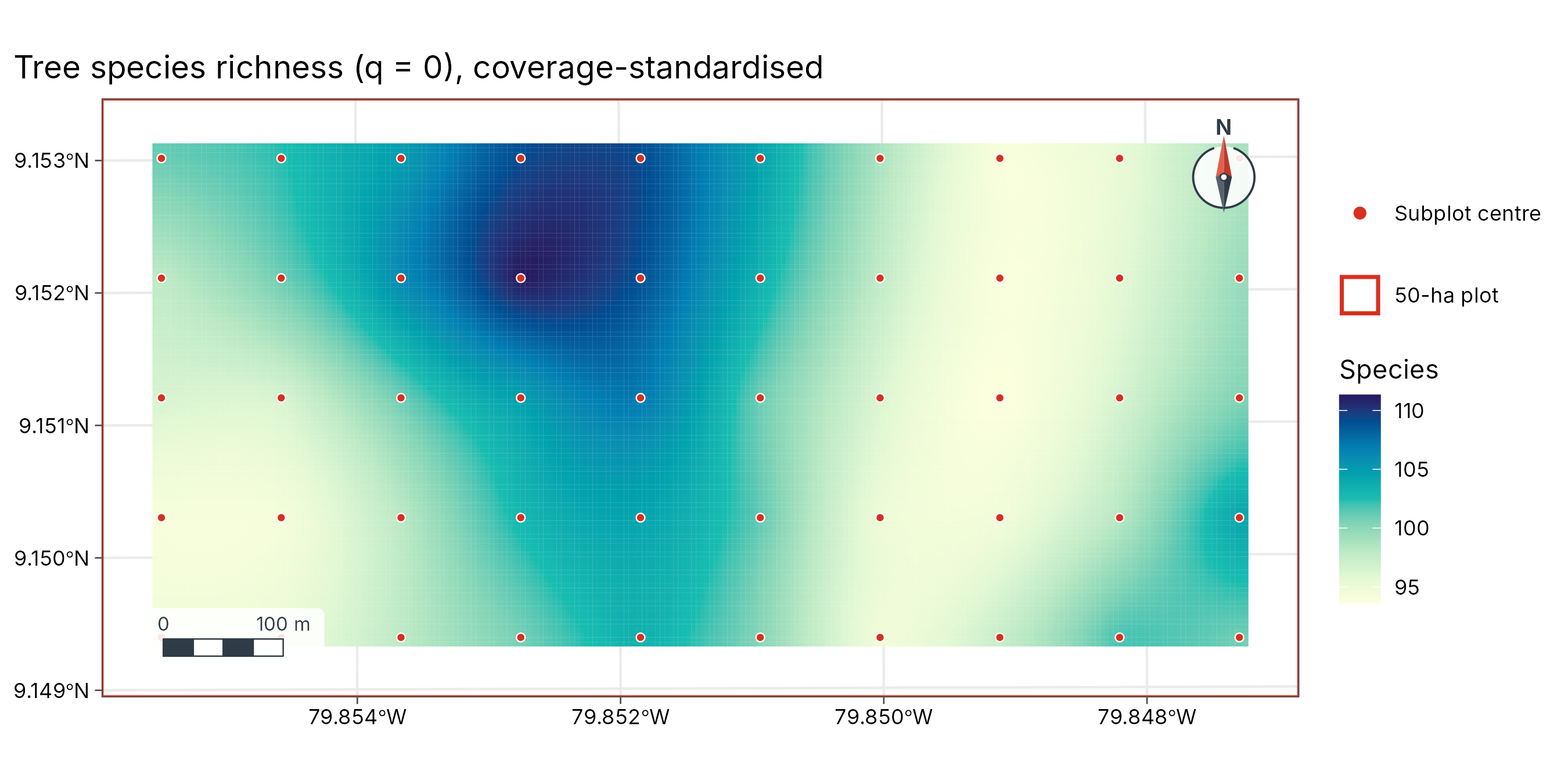

Is diversity clustered?

Moran’s I on the subplot richness, and local hot and cold spots.

pts <- sf::st_transform(centres, 4326) |> left_join(rich, by = "plot")
xy <- sf::st_coordinates(pts)
pts_df <- tibble::tibble(plot = pts$plot, richness = pts$richness, lon = xy[, 1], lat = xy[, 2])
geo_moran(pts_df, richness, lon, lat)
#> # A tibble: 1 × 7
#>   statistic expectation variance p.value     n nperm method                     
#>       <dbl>       <dbl>    <dbl>   <dbl> <int> <dbl> <chr>                      
#> 1    0.0135     -0.0204 0.000349   0.051    50   999 Moran's I (inverse-distanc…
geo_hotspot(pts_df, richness, k = 4) |> count(hotspot)
#> # A tibble: 2 × 2
#>   hotspot             n
#>   <fct>           <int>
#> 1 hot                 6
#> 2 not significant    44

References

Condit R, Pitman N, Leigh EG, et al. (2002) Beta-diversity in tropical forest trees. Science 295: 666-669.