2. Cartography concepts: projections, classes and colour

A map is a model of the world, not a picture of it. Three decisions change what readers conclude from a thematic map: the projection (which distortions you accept), the classification (how numbers are grouped into colours) and the colour scheme (what the colours imply). This chapter explains the theory behind each, shows how tidymapr chooses, and how to justify the choice in a methods section.

library(tidymapr)
library(dplyr)
world <- sf::st_read(system.file("shapes/world.gpkg", package = "spData"), quiet = TRUE)

The data are life expectancy at birth (years) for 177 countries, from the spData package.

1. Coordinate reference systems and projections

The concept

Positions on the Earth are angles (longitude and latitude) on a curved surface. A coordinate reference system (CRS) says how those numbers relate to real places: the datum (the model of the Earth’s shape, e.g. WGS84) and, for flat maps, the projection (the mathematical rule that flattens the curved surface onto a plane).

Flattening a sphere always distorts something. Gauss’s Theorema Egregium (1827) proves that no flat map can keep both areas and angles correct everywhere. Each projection chooses what to keep:

Property kept	Name	Use it for	Examples
Area	Equal-area	Any map of densities, rates or amounts per area; choropleths	Equal Earth, Mollweide, Lambert azimuthal equal-area (LAEA), Albers
Angles and local shapes	Conformal	Navigation, web tiles, small study areas	Mercator, UTM, Lambert conformal conic
Distances from one point	Equidistant	Ranges from a site or a city	Azimuthal equidistant
A compromise	None exactly	General world reference maps	Robinson, Winkel Tripel

Mercator is conformal, so it exaggerates areas towards the poles: Greenland looks as large as Africa, which is 14 times bigger. On a choropleth this inflates the visual weight of high-latitude countries, so use an equal-area projection whenever colour represents a quantity.

The same data in four projections

# Antarctica is left out: Mercator cannot show the poles at all
no_antarctica <- world[world$continent != "Antarctica", ]
p <- function(proj, label) {
  plot_choropleth(no_antarctica, lifeExp, n = 5, style = "jenks", legend_title = "Years") +
    coord_projection(proj) +
    ggplot2::labs(title = label)
}
geo_panels(
  p("equal_earth", "Equal Earth (equal-area)"),
  p("mercator", "Mercator (conformal)"),
  p("mollweide", "Mollweide (equal-area)"),
  p("robinson", "Robinson (compromise)"),
  ncol = 2, guides = "collect"
)

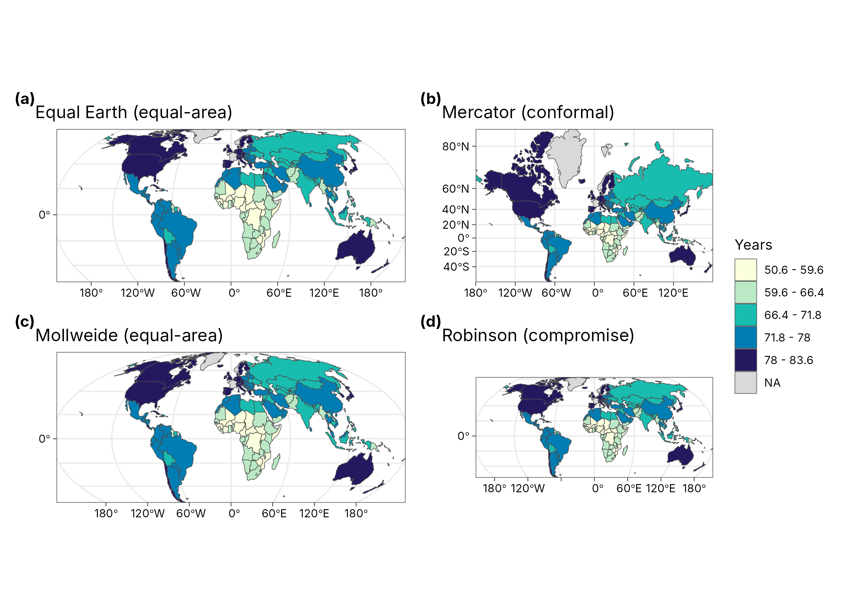
How to read it. The colours are identical in all four panels; only the geometry changes. Compare Russia, Canada and Greenland with Africa: in Mercator they dominate the map, in the equal-area projections they take their true share of the page.

How tidymapr chooses (geo_crs(), geo_automap()):

Extent of your data	Projection chosen	Why
The whole world	Equal Earth	Equal-area, with a natural look (Šavrič et al. 2019)
A continent or large region	Lambert azimuthal equal-area, centred on the data	Equal-area, least distortion near the centre
A study area (a few degrees)	Local UTM zone	Conformal and nearly equal-area at this scale; metres for scale bars
Raster tiles or interpolated surfaces	Longitude-latitude	Avoids resampling the grid

You can always override it: geo_map(crs = "laea"), crs = 32755 (an EPSG code) or + coord_projection("mollweide").

2. Classifying numbers into map classes

The concept

A choropleth shows numbers as colours. Readers can tell apart only about five to seven shades of one hue, so values are grouped into classes. How the class breaks are drawn changes the map’s message. The standard methods:

Style	Rule	Good for	Risk
"equal"	Equal-width intervals over the range	Familiar units (e.g. 0-10 °C, 10-20 °C)	One outlier squeezes all other values into one class
"quantile"	Equal numbers of features per class	Ranking; showing relative position	Very different values can share a class; similar values split
"jenks"	Natural breaks: minimise the variance within classes (Fisher 1958; Jenks 1967)	Clustered or skewed data; the general default	Breaks are data-specific, so two maps are not directly comparable
"pretty"	Rounded breaks	Readable legends	Classes may be uneven
"sd"	Mean ± whole standard deviations	Showing departure from average	Needs a roughly symmetric distribution

The goodness of variance fit (GVF) measures how well classes describe the data: GVF = 1 − (sum of squared deviations from class means) / (sum of squared deviations from the overall mean). GVF = 1 means classes explain all the variation; values above about 0.8 are good.

The same data, four classifications

styles <- c(equal = "Equal interval", quantile = "Quantile", jenks = "Natural breaks (Jenks)", sd = "Standard deviation")
maps <- lapply(names(styles), function(s) {
  plot_choropleth(world, lifeExp, n = 5, style = s, legend_title = "Years") +
    ggplot2::labs(title = styles[[s]])
})
geo_panels(maps, ncol = 2, guides = "keep")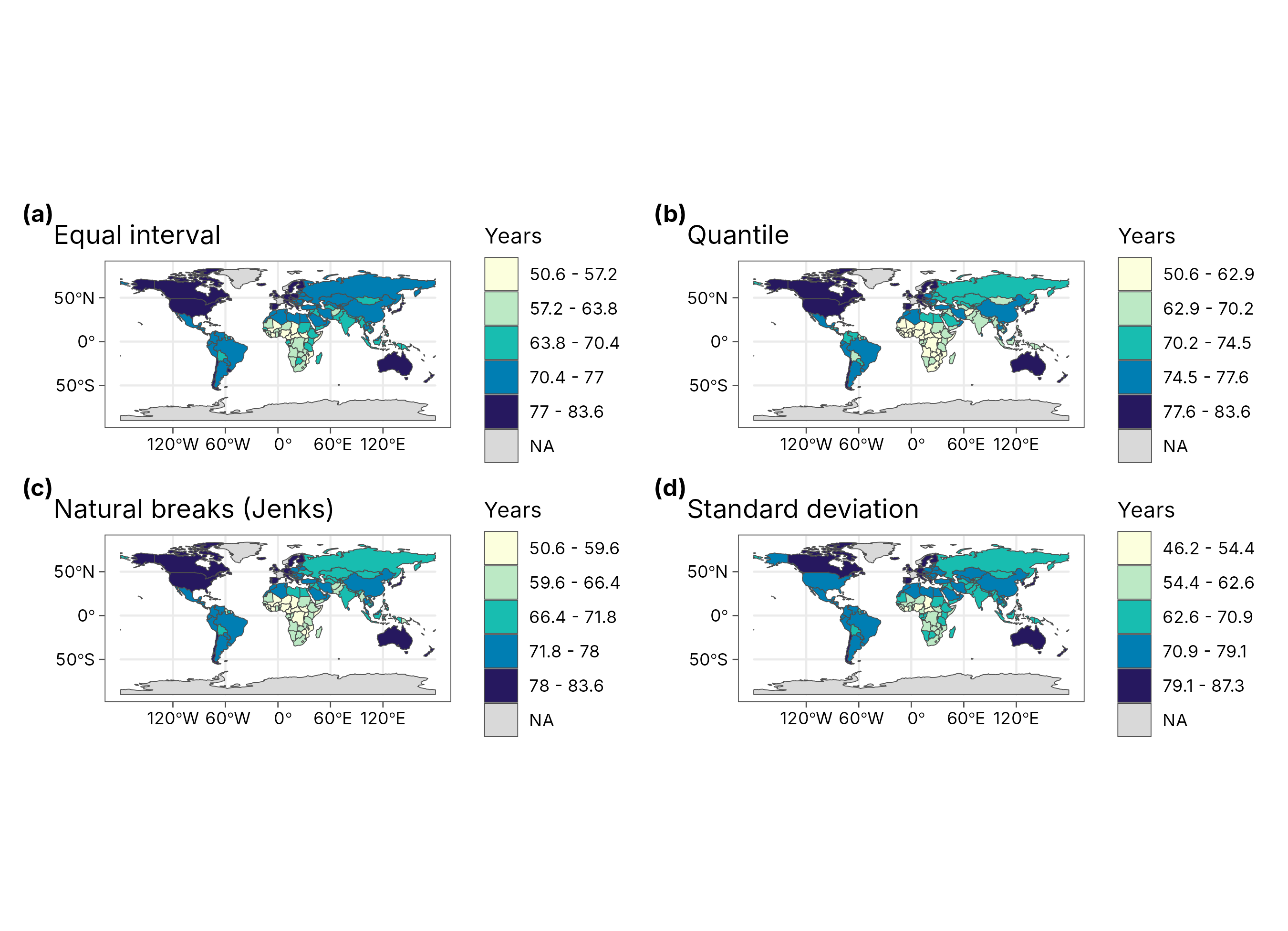

gvf <- lapply(names(styles), function(s) {
  cl <- attr(geo_classify(world, lifeExp, n = 5, style = s), "classification")
  tibble(
    style = styles[[s]],
    breaks = paste(round(cl$breaks, 1), collapse = ", "),
    countries_per_class = paste(cl$counts, collapse = " / "),
    GVF = round(cl$gvf, 3)
  )
})
knitr::kable(bind_rows(gvf), caption = "Class breaks, class sizes and goodness of variance fit for life expectancy (5 classes).")

Class breaks, class sizes and goodness of variance fit for life expectancy (5 classes).

style	breaks	countries_per_class	GVF
Equal interval	50.6, 57.2, 63.8, 70.4, 77, 83.6	15 / 21 / 31 / 61 / 39	0.943
Quantile	50.6, 62.9, 70.2, 74.5, 77.6, 83.6	34 / 33 / 33 / 33 / 34	0.933
Natural breaks (Jenks)	50.6, 59.6, 66.4, 71.8, 78, 83.6	22 / 30 / 31 / 53 / 31	0.955
Standard deviation	46.2, 54.4, 62.6, 70.9, 79.1, 87.3	6 / 25 / 40 / 67 / 29	0.937

How to interpret this table. Natural breaks have the highest GVF: they follow the gaps in the data. Quantiles put roughly the same number of countries in each class, so the darkest class always covers a fifth of the map whatever the values. Equal intervals and standard deviations follow the scale of the numbers, so they are easy to explain but leave some classes almost empty.

How tidymapr chooses. geo_automap() looks at the shape of the distribution: equal intervals when it is roughly symmetric, natural breaks when it is skewed, quantiles when it is heavy-tailed; five classes for 30 or more features, fewer for small samples. It never uses a continuous colour ramp for polygons, because readers cannot judge exact values from a continuous ramp.

3. Colour schemes

Scheme	Shape	Use for	tidymapr palettes
Sequential	Light to dark, one or two hues	Amounts from low to high (density, richness, elevation)	"YlOrRd", "Blues 3", "YlGnBu", "viridis"
Diverging	Two hues meeting at a neutral midpoint	Departures from a meaningful centre (change, anomaly, residual)	"RdBu", "Blue-Red"
Qualitative	Distinct hues of equal weight	Categories with no order (land cover, species, clusters)	Okabe-Ito colours

Rules that tidymapr follows: darker means more; a diverging scheme only when zero (or another centre) means something; palettes safe for colour vision deficiency (viridis, Okabe-Ito and ColorBrewer sequential schemes are). geo_automap() picks the ramp from the field’s meaning: blues for water, greens for vegetation, viridis for elevation, and a diverging ramp for data that cross zero.

4. Map elements

Element	When it belongs	When to leave it out
Scale bar	Regional and local maps	World maps: scale changes across the map, so one bar would mislead
North arrow	Local maps, field maps	World maps, and maps where north is obviously up
Graticule (lines of latitude and longitude)	World and continental maps, to show the projection	Small study areas
Legend	Always, with units	Never omit it
Source and date	Always (caption)	Never omit it

tidymapr places the scale bar and north arrow in the emptiest corners, and drops them on world maps.

5. Let tidymapr choose, and explain

m <- geo_automap(world, lifeExp, legend_title = "Life expectancy (years)")
m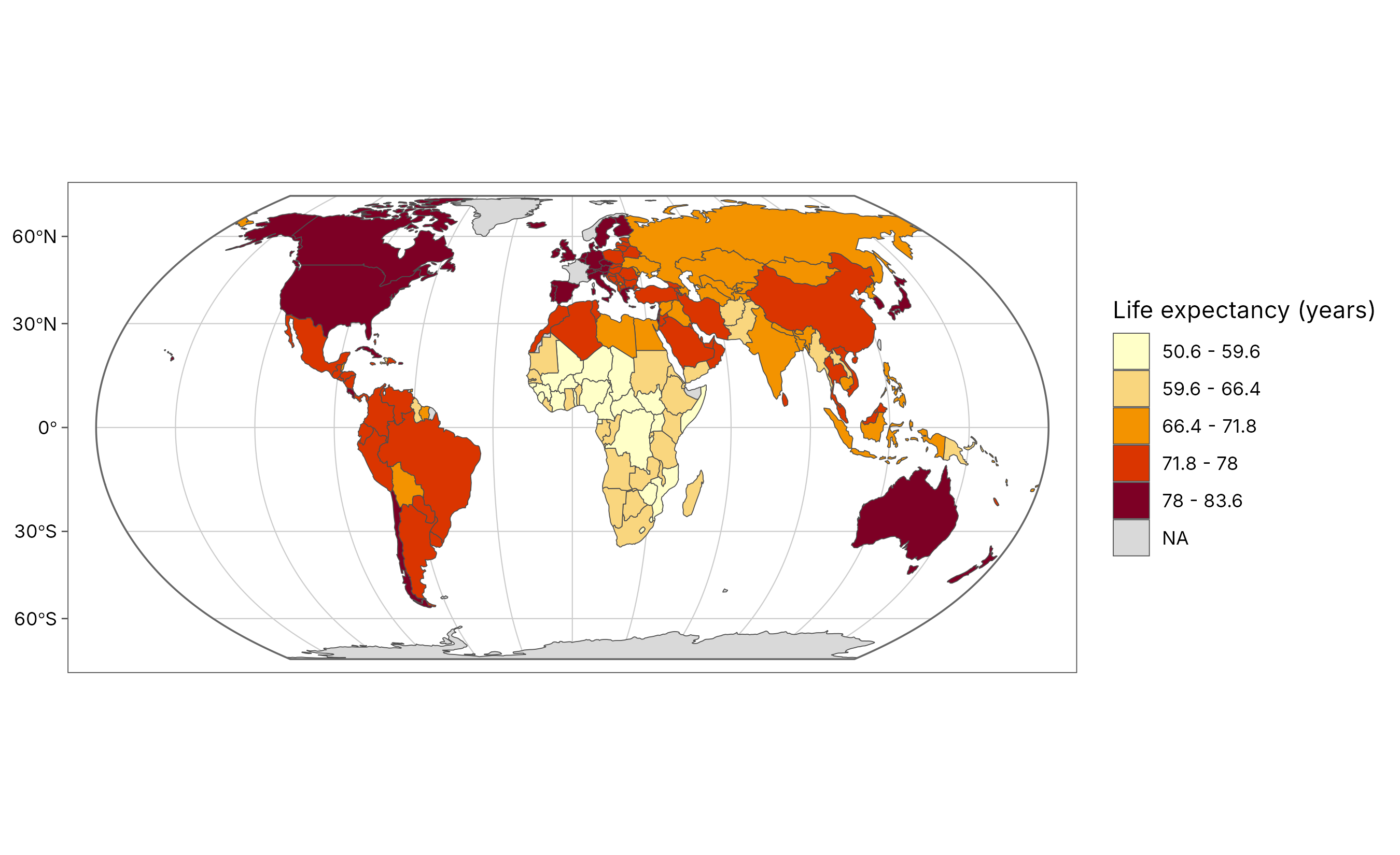

knitr::kable(geo_automap_explain(m), caption = "Every design decision behind the map above, with its reason.")

Every design decision behind the map above, with its reason.

element	choice	reason
projection	equal_earth	Data span 360 degrees: a world map; Equal Earth keeps true areas.
symbology	graduated colours (jenks, 5 classes, YlOrRd)	‘lifeExp’ is numeric and left-skewed (n = 167, skew -0.5), so natural breaks (Jenks) in 5 classes; ramp: general quantity: yellow-orange-red. Goodness of variance fit 0.95.
basemap	none	Polygons, rasters and large extents need no basemap.
graticule	30 degrees, world outline	World map: graticule and outline show the projection.
scale bar	none	Scale varies across a world map, so a single bar would mislead.

How to report it. The table is written to be pasted into a methods section. For example:

Maps were drawn with tidymapr (Moses 2026) in R. Life expectancy was mapped in the Equal Earth projection, which preserves area, using five natural-breaks classes (Fisher-Jenks; goodness of variance fit 0.95) and a sequential yellow-orange-red palette.

References

Fisher, W. D. (1958). On grouping for maximum homogeneity. Journal of the American Statistical Association, 53, 789-798.

Jenks, G. F. (1967). The data model concept in statistical mapping. International Yearbook of Cartography, 7, 186-190.

Šavrič, B., Patterson, T. and Jenny, B. (2019). The Equal Earth map projection. International Journal of Geographical Information Science, 33, 454-465.

Snyder, J. P. (1987). Map Projections: A Working Manual. US Geological Survey Professional Paper 1395.

Brewer, C. A. (2016). Designing Better Maps: A Guide for GIS Users, 2nd edition. Esri Press.