3. Spatial autocorrelation: Moran's I, LISA and hot spots • tidymapr

The concept

“Everything is related to everything else, but near things are more related than distant things.” (Tobler 1970)

Spatial autocorrelation is the degree to which values at nearby places resemble each other. It matters for two reasons:

It is often the finding. Clusters of disease, pollution, species richness or poverty are what we want to locate.
It breaks ordinary statistics. Nearby samples are not independent, so a regression or t-test on spatial data overstates the evidence (too-small p-values) unless the autocorrelation is accounted for.

Two questions, two kinds of statistic:

Question	Statistic	Scale	tidymapr
Is there clustering anywhere in the study area?	Moran’s I	Global: one number	`geo_moran()`
Where are the clusters and outliers?	Local Moran’s I (LISA)	Local: one value per site	`geo_lisa()`
Where are the hot and cold spots?	Getis-Ord Gi*	Local: one value per site	`geo_hotspot()`

library(tidymapr)
library(dplyr)

The data

Zinc concentration (ppm) in 155 topsoil samples from the floodplain of the river Meuse, the Netherlands (Rikken and Van Rijn 1993), shipped with terra. Heavy metals arrive with flood water, so we expect high values near the river.

meuse <- terra::unwrap(readRDS(system.file("ex/meuse.rds", package = "terra")))
samples <- sf::st_as_sf(as.data.frame(meuse), coords = c("x", "y"), crs = 28992)
samples$log_zinc <- log(samples$zinc)
summary(samples$zinc)
#>    Min. 1st Qu.  Median    Mean 3rd Qu.    Max. 
#>   113.0   198.0   326.0   469.7   674.5  1839.0

Zinc is strongly right-skewed (the mean is well above the median), so we analyse its logarithm: these statistics compare values with their mean, and a few extreme values would otherwise dominate.

1. Global Moran’s I

Theory

$I = \frac{n}{\sum_i \sum_j w_{ij}} \; \frac{\sum_i \sum_j w_{ij} (x_i - \bar{x})(x_j - \bar{x})}{\sum_i (x_i - \bar{x})^2}$

$x_i$ is the value at site $i$ , $\bar{x}$ the mean and $w_{ij}$ the spatial weight between sites $i$ and $j$ ; tidymapr uses inverse distance, $w_{ij} = 1 / d_{ij}$ , so close pairs count most. The numerator adds up the products of deviations for neighbouring pairs: it is large and positive when neighbours deviate from the mean in the same direction.

Value of I	Meaning
Clearly above $E[I] = -1/(n-1)$ (close to 0)	Positive autocorrelation: similar values cluster
Close to $E[I]$	No spatial pattern: values are arranged as if at random
Below $E[I]$	Negative autocorrelation: neighbours differ (a checkerboard)

Moran’s I is not bounded by −1 and 1 like a correlation, and its size depends on the weights, so judge it against its expectation and its permutation p-value: the values are shuffled among the sites 999 times, and the p-value is the share of shuffles giving an I at least as extreme as the observed one.

Run it

m <- geo_moran(samples, log_zinc, nperm = 999, correlogram = TRUE, bins = 8, seed = 1)
m
#> # A tibble: 1 × 7
#>   statistic expectation variance p.value     n nperm method                     
#>       <dbl>       <dbl>    <dbl>   <dbl> <int> <dbl> <chr>                      
#> 1     0.119    -0.00649 0.000113   0.001   155   999 Moran's I (inverse-distanc…

Interpretation. I = 0.119 against an expectation of -0.0065 under randomness, with a permutation p-value of 0.001. Log zinc is positively autocorrelated: samples near each other have similar concentrations.

The correlogram: over what distance?

The correlogram computes Moran’s I separately for pairs in successive distance bands. It shows the range of the pattern: the distance up to which neighbours resemble each other.

cg <- attr(m, "correlogram")
knitr::kable(cg, digits = 3, caption = "Moran's I by distance band (distance in metres, n = number of pairs).")

Moran’s I by distance band (distance in metres, n = number of pairs).
bin	distance	moran	n
1	303.485	0.290	1492
2	622.335	-0.031	1492
3	901.330	-0.169	1492
4	1202.768	-0.112	1492
5	1554.735	-0.023	1491
6	1956.427	0.038	1492
7	2494.927	-0.051	1492
8	3323.580	0.007	1492


ggplot2::ggplot(cg, ggplot2::aes(distance, moran)) +
  ggplot2::geom_hline(yintercept = 0, colour = "grey50") +
  ggplot2::geom_line(colour = "#349295") +
  ggplot2::geom_point(colour = "#349295", size = 2.5) +
  ggplot2::labs(x = "Distance between samples (m)", y = "Moran's I") +
  theme_tidymapr()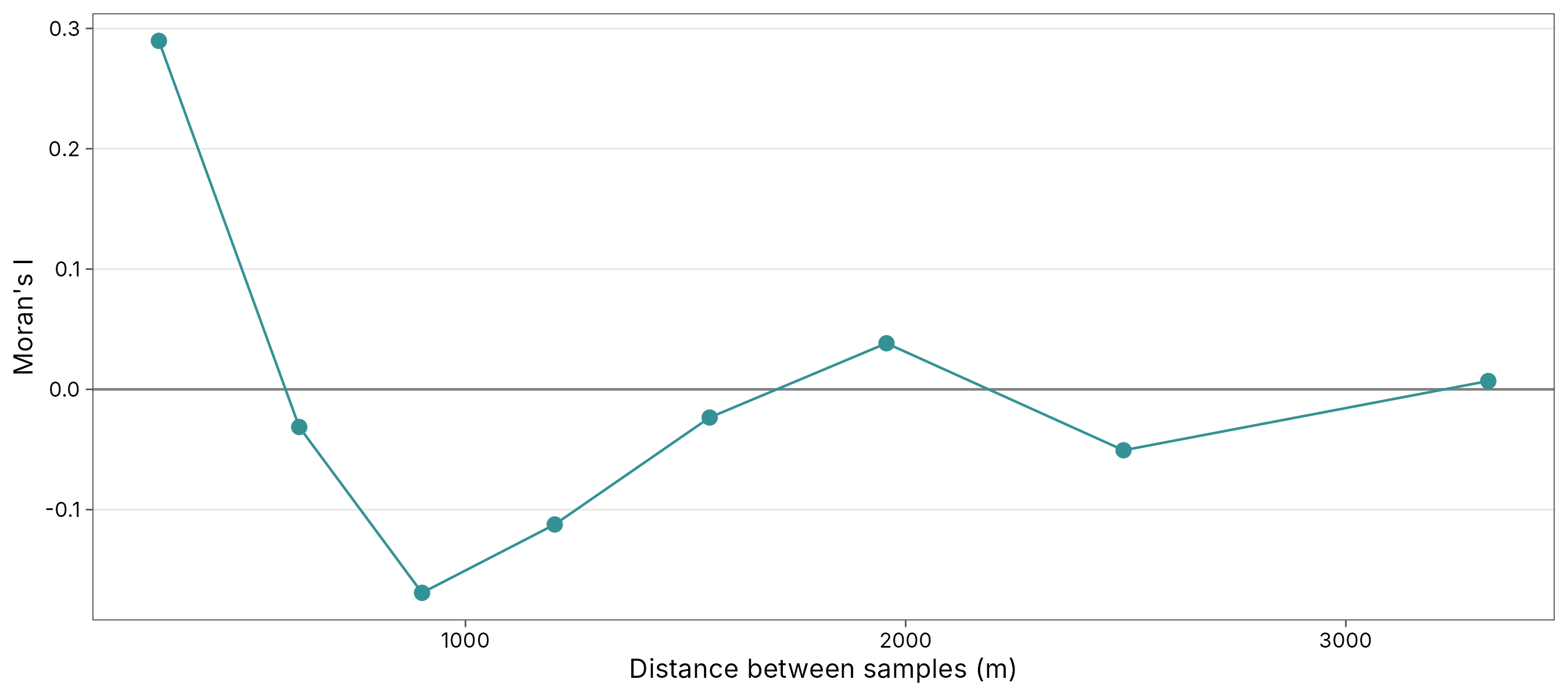

Moran's I correlogram of log zinc: positive at short distances, falling to zero and below with distance

Interpretation. Moran’s I is highest in the first band (about 303 m) and falls to zero within about 600 m. Beyond that, samples are no more alike than random pairs; negative values at middle distances reflect the contrast between the river bank and the inland floodplain. This range is useful later: it tells kriging (Chapter 4) how far to look for neighbours.

2. Local Moran’s I (LISA)

Theory

Anselin (1995) split global Moran’s I into a contribution from each site:

$I_i = \frac{x_i - \bar{x}}{s^2} \sum_j w_{ij} (x_j - \bar{x})$

The sum is the spatial lag: the weighted average deviation of site $i$ ’s neighbours (here, its k = 8 nearest neighbours). Comparing the site with its neighbourhood gives four types, tested by conditional permutation:

Cluster	Site	Neighbours	Meaning
High-High	High	High	Core of a hot cluster
Low-Low	Low	Low	Core of a cold cluster
High-Low	High	Low	Spatial outlier: a high value among low ones
Low-High	Low	High	Spatial outlier: a low value among high ones
not significant			No evidence of local pattern

lisa <- geo_lisa(samples, log_zinc, k = 8, nperm = 999, seed = 1)
knitr::kable(count(sf::st_drop_geometry(lisa), cluster), caption = "Number of samples in each LISA class.")

Number of samples in each LISA class.
cluster	n
High-High	23
Low-Low	31
High-Low	3
Low-High	1
not significant	97


geo_map(title = "Local Moran's I clusters of log zinc", caption = "Data: terra package; 8 nearest neighbours, 999 permutations") |>
  map_points(lisa, fill = cluster, group = "LISA cluster", size = 2.2,
    palette = c("High-High" = "#B2182B", "Low-Low" = "#2166AC", "High-Low" = "#F4A582",
                "Low-High" = "#92C5DE", "not significant" = "grey85"))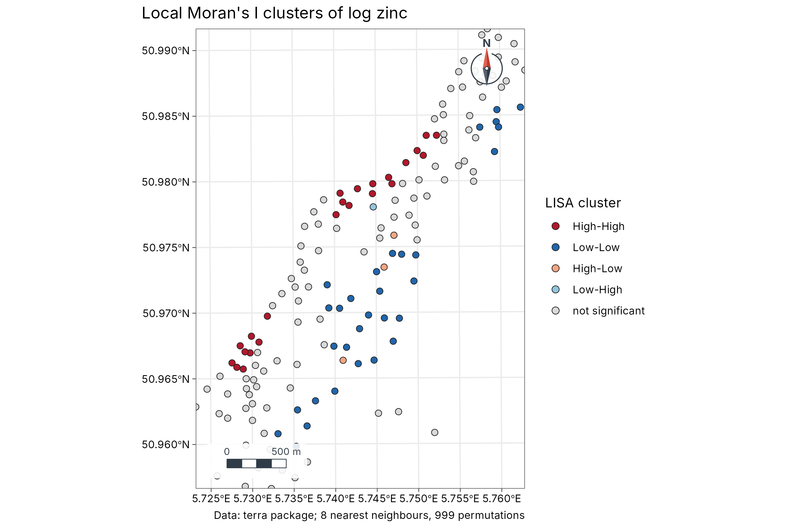

Map of LISA clusters for log zinc along the river Meuse

Interpretation. The High-High cluster lies along the north-western edge of the sampled area, on the bank of the Meuse: the soils flooded most often. The Low-Low cluster lies further from the river, to the south-east. The hot and cold spots below show the same split. The few outliers mark local disturbances or measurement differences and deserve a closer look.

3. Getis-Ord Gi* hot spots

Theory

Getis and Ord (1992) compare the sum of values in each site’s neighbourhood (including the site itself, hence the star) with what is expected if values were spread at random:

$G_i^* = \frac{\sum_j w_{ij} x_j - \bar{x} \sum_j w_{ij}} {s \sqrt{\left[n \sum_j w_{ij}^2 - \left(\sum_j w_{ij}\right)^2\right] / (n-1)}}$

$G_i^*$ is a z-score: above +1.96 is a hot spot and below −1.96 a cold spot at the 5 % level. Unlike LISA, Gi* does not detect outliers; it answers only “is this area high or low overall?”, which makes it easier to explain to non-specialists.

hot <- geo_hotspot(samples, log_zinc, k = 8)
knitr::kable(count(sf::st_drop_geometry(hot), hotspot), caption = "Hot and cold spots (Gi*, 5 % level).")

Hot and cold spots (Gi*, 5 % level).
hotspot	n
hot	31
cold	39
not significant	85


geo_map(title = "Hot spots of zinc (Getis-Ord Gi*)", caption = "Data: terra package; 8 nearest neighbours") |>
  map_points(hot, fill = hotspot, group = "Gi*", size = 2.2,
    palette = c(hot = "#B2182B", cold = "#2166AC", "not significant" = "grey85"))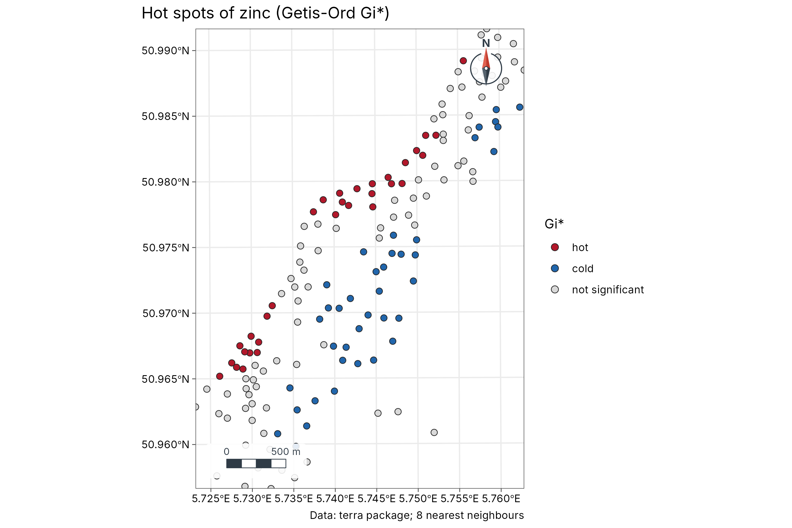

Map of Getis-Ord hot and cold spots of zinc

Choosing neighbours and handling many tests

Choice	Effect	Advice
`k` nearest neighbours	Every site has the same number of neighbours	Good default for irregular samples; try `k` from 4 to 12 and check the result is stable
`dist` (a distance band)	Neighbours within a fixed distance	Use when the process has a known reach, e.g. the correlogram’s range
Many local tests	With 155 tests at the 5 % level, about 8 can be “significant” by chance	Lower `alpha` (e.g. 0.01) or describe clusters, not single points

How to report it

Log-transformed zinc showed significant positive spatial autocorrelation (Moran’s I = 0.12, inverse-distance weights, permutation p = 0.001, 999 permutations). The correlogram showed autocorrelation up to about 600 m. Local Moran’s I (8 nearest neighbours) identified 23 samples in High-High clusters along the river and 31 in Low-Low clusters inland. Analyses used tidymapr, whose statistics equal spdep’s.

References

Anselin, L. (1995). Local indicators of spatial association: LISA. Geographical Analysis, 27, 93-115.

Getis, A. and Ord, J. K. (1992). The analysis of spatial association by use of distance statistics. Geographical Analysis, 24, 189-206.

Moran, P. A. P. (1950). Notes on continuous stochastic phenomena. Biometrika, 37, 17-23.

Rikken, M. G. J. and Van Rijn, R. P. G. (1993). Soil pollution with heavy metals. MSc thesis, Utrecht University.

Tobler, W. R. (1970). A computer movie simulating urban growth in the Detroit region. Economic Geography, 46, 234-240.