7. Point clusters and landscape fragmentation

library(tidymapr)
library(dplyr)
world <- sf::st_read(system.file("shapes/world.gpkg", package = "spData"), quiet = TRUE)

Part A. Clusters of points: DBSCAN

The concept

Many data sets are events at locations: earthquakes, disease cases, crimes, animal sightings, fires. A common question is whether they form groups, and where. Chapter 3’s statistics test values at fixed sites; here the locations are the data.

DBSCAN (density-based spatial clustering of applications with noise; Ester et al. 1996) finds groups as regions where points are dense, separated by sparse regions. Unlike k-means it does not need the number of clusters in advance, finds clusters of any shape, and labels isolated points as noise instead of forcing them into a group.

Term	Definition
eps (ε)	The neighbourhood radius. tidymapr measures it in metres on the ground, also for longitude/latitude data
min_pts	Minimum number of points within ε for a point to be a core point
Core point	Has at least min_pts points (itself included) within ε
Border point	Within ε of a core point but not a core point itself
Noise (cluster 0)	Neither: an isolated event
Cluster	Core points linked through chains of neighbours, plus their border points

Earthquakes near Fiji

1000 earthquakes of magnitude 4 or more near Fiji since 1964 (Harvard PRIM-H project), in R’s datasets package.

cl <- geo_dbscan(datasets::quakes, eps = 50000, min_pts = 15, lon = long, lat = lat)
cl$group <- factor(ifelse(cl$cluster == 0, "Noise", paste("Cluster", cl$cluster)),
  levels = c(paste("Cluster", sort(unique(cl$cluster[cl$cluster > 0]))), "Noise"))

summary_tbl <- sf::st_drop_geometry(cl) |>
  summarise(events = n(), core = sum(core), mean_depth_km = round(mean(depth)),
            mean_magnitude = round(mean(mag), 2), .by = group) |>
  arrange(group)
knitr::kable(summary_tbl, caption = "Clusters found by DBSCAN (eps = 50 km, min_pts = 15).")

Clusters found by DBSCAN (eps = 50 km, min_pts = 15).

group	events	core	mean_depth_km	mean_magnitude
Cluster 1	259	223	554	4.49
Cluster 2	23	10	225	4.47
Cluster 3	25	15	102	4.70
Cluster 4	76	57	518	4.56
Cluster 5	19	7	217	4.44
Cluster 6	26	15	217	4.57
Cluster 7	17	3	98	4.68
Cluster 8	27	11	88	4.64
Cluster 9	15	1	63	4.90
Noise	513	0	207	4.69

land <- suppressWarnings(sf::st_crop(sf::st_shift_longitude(world), c(xmin = 160, ymin = -40, xmax = 190, ymax = -8)))
geo_map(
  title = "Earthquake clusters near Fiji (DBSCAN, 50 km, 15 events)",
  caption = "Data: datasets::quakes; land: spData",
  crs = "+proj=laea +lat_0=-22 +lon_0=178 +datum=WGS84 +units=m"
) |>
  map_polygons(land, fill = "grey88", border = "grey60", label = "Land") |>
  map_polygons(attr(cl, "hulls"), fill = NA, border = "grey20", label = "Cluster outlines", linewidth = 0.4) |>
  map_points(cl, fill = group, group = "Events", size = 1.4,
    palette = c(grDevices::hcl.colors(nlevels(cl$group) - 1, "Dark 3"), "grey80"))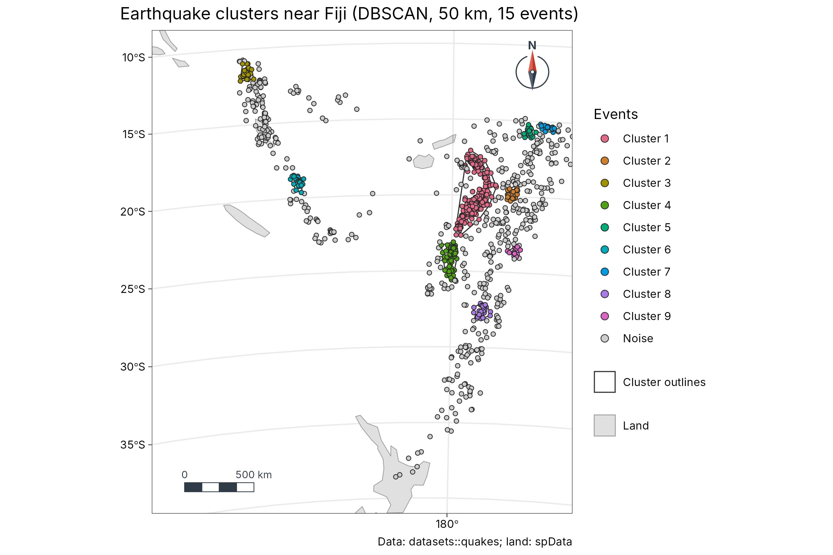

Interpretation. 487 of 1000 events (49 %) fall in 9 dense clusters; the rest are noise. The table adds meaning: the largest cluster (259 events) is deep, averaging 554 km below the surface, while the smaller clusters lie between 63 and 518 km. These are earthquakes within the Pacific plate as it sinks beneath the Tonga-Fiji region; DBSCAN separates its deep and shallower seismic zones using location alone.

Choosing eps and min_pts

Setting	Too small	Too large
eps	Most points become noise; real clusters break apart	Separate clusters merge into one
min_pts	Chance groupings become clusters	Only the densest cores survive

Choose eps from the process (the reach of an interaction, the correlogram range of Chapter 3), or plot each point’s distance to its min_pts-th nearest neighbour sorted from smallest to largest, and take the distance at the “knee” where the curve bends up. A common start is min_pts = 2 × the number of dimensions, and larger for noisy data. Always report both settings, and check that the main conclusions hold for nearby values.

Part B. Landscape fragmentation

The concept

Habitat loss is often accompanied by fragmentation: the remaining habitat is broken into smaller, more isolated pieces with more edge. Landscape metrics quantify this from a categorical raster (land cover, habitat / non-habitat). tidymapr computes the standard FRAGSTATS metrics (McGarigal and Marks 1995), building patches with the 8-neighbour rule. Its results equal landscapemetrics’ on projected rasters; unlike it, tidymapr measures longitude/latitude rasters in true hectares and metres.

A two-class landscape

We use the vegetation classes from Chapter 6: Sentinel-2 NDVI above and below the Otsu threshold, over Luxembourg.

s2 <- terra::rast(system.file("ex/sent2_L2A_2024-08-24.tif", package = "terra"))
ndvi <- geo_spectral_index(s2, "NDVI", threshold = "otsu")
cover <- terra::ifel(ndvi[["above"]], 2, 1)
names(cover) <- "class"     # 1 = low vegetation, 2 = high vegetation

cls <- geo_landscape(cover, level = "class") |>
  mutate(class = c("1" = "Low vegetation", "2" = "High vegetation")[as.character(class)])
knitr::kable(cls, digits = 1, caption = "Class-level landscape metrics.")

Class-level landscape metrics.

class	np	ca	pland	lpi	area_mn	ed	ai	mesh
Low vegetation	161	39518.4	14.6	2.0	245.5	4.4	43.3	241.7
High vegetation	8	231760.8	85.4	85.1	28970.1	4.4	89.4	196569.6

Metric	Name	Units	Meaning	Fragmented habitat has
np	Number of patches	count	Separate pieces of the class	More patches
ca	Class area	ha	Total area of the class	—
pland	Percentage of landscape	%	Share of the map	—
lpi	Largest patch index	%	The largest patch as a share of the whole map	Lower LPI
area_mn	Mean patch area	ha	Average patch size	Smaller patches
ed	Edge density	m/ha	Length of class edge per hectare of landscape	More edge
ai	Aggregation index	%	How often cells of the class touch each other, relative to the most compact possible arrangement	Lower AI
mesh	Effective mesh size	ha	Expected size of the patch containing a random point (Jaeger 2000)	Smaller mesh

Interpretation. High vegetation covers 85 % of the landscape, mostly in one large connected patch (largest patch index 85 %, effective mesh size 196,570 ha). Low vegetation is split into 161 small patches with a mean size of 245 ha and a lower aggregation index: it is the fragmented class. In words: green cover forms the matrix of this late-summer landscape, with towns, roads and harvested fields as scattered gaps.

knitr::kable(geo_landscape(cover, level = "landscape"), digits = 3,
  caption = "Landscape-level metrics: total patches, area, edge density, Shannon (shdi) and Simpson (sidi) diversity of classes, and effective mesh size.")

Landscape-level metrics: total patches, area, edge density, Shannon (shdi) and Simpson (sidi) diversity of classes, and effective mesh size.

np	ta	ed	shdi	sidi	mesh
169	271279.2	4.423	0.415	0.249	196811.3

shdi (Shannon’s diversity index) and sidi (Simpson’s) describe how many classes there are and how evenly they share the map. They reach their maximum when all classes cover equal areas, and are useful for comparing landscapes or the same landscape over time.

Cautions

• Metrics depend on resolution and extent. Patches merge or split when cells are coarser or finer, so compare landscapes only at the same resolution and extent (the modifiable areal unit problem).
• Classification comes first. A small change in the NDVI cut changes every metric; report how classes were made.
• Many metrics are correlated. Choose a few that answer your question, for example pland (how much), np or area_mn (how broken) and ai or mesh (how connected).

How to report it

Landscape metrics were computed with tidymapr (8-neighbour patches) from a two-class map of Sentinel-2 NDVI (24 August 2024) thresholded by Otsu’s method at 0.45. High vegetation covered 85 % of the landscape, with a largest patch index of 85 %.

References

Ester, M., Kriegel, H.-P., Sander, J. and Xu, X. (1996). A density-based algorithm for discovering clusters in large spatial databases with noise. Proceedings of KDD-96, 226-231.

Hesselbarth, M. H. K. et al. (2019). landscapemetrics: an open-source R tool to calculate landscape metrics. Ecography, 42, 1648-1657.

Jaeger, J. A. G. (2000). Landscape division, splitting index, and effective mesh size. Landscape Ecology, 15, 115-130.

McGarigal, K. and Marks, B. J. (1995). FRAGSTATS: spatial pattern analysis program for quantifying landscape structure. USDA Forest Service General Technical Report PNW-351.