
Spatial analysis
geospatial.RmdThe analysis tools of a desktop GIS, written in C++ and run on several cores, each checked against the reference R package. Every example uses real data shipped with R packages.
Interpolation: kriging and IDW
Zinc in the floodplain soils of the river Meuse (155 samples, shipped
with terra). geo_interpolate() krigs with a fitted
variogram; its results equal gstat’s to machine precision.
meuse <- terra::unwrap(readRDS(system.file("ex/meuse.rds", package = "terra")))
samples <- sf::st_as_sf(as.data.frame(meuse), coords = c("x", "y"), crs = 28992)
samples$log_zinc <- log(samples$zinc)

grid <- terra::rast(terra::ext(terra::vect(samples)) + 100, resolution = 20, crs = "EPSG:28992")
zinc <- geo_interpolate(samples, log_zinc, grid, method = "kriging", name = "log_zinc")
zinc
#> class       : SpatRaster
#> size        : 205, 149, 2  (nrow, ncol, nlyr)
#> resolution  : 20.03356, 19.98537  (x, y)
#> extent      : 178505, 181490, 329614, 333711  (xmin, xmax, ymin, ymax)
#> coord. ref. : Amersfoort / RD New (EPSG:28992)
#> source(s)   : memory
#> names       : log_zinc, variance
#> min values  : 4.735424,  0.00156
#> max values  : 7.541052, 0.791856
geo_map(title = "Zinc in Meuse floodplain soils (kriged)", caption = "Data: terra package") |>
  map_raster(exp(zinc[["log_zinc"]]), name = "Zinc (ppm)", palette = "YlOrRd") |>
  map_points(samples, preset = "sample_site", label = "Samples", size = 1.3)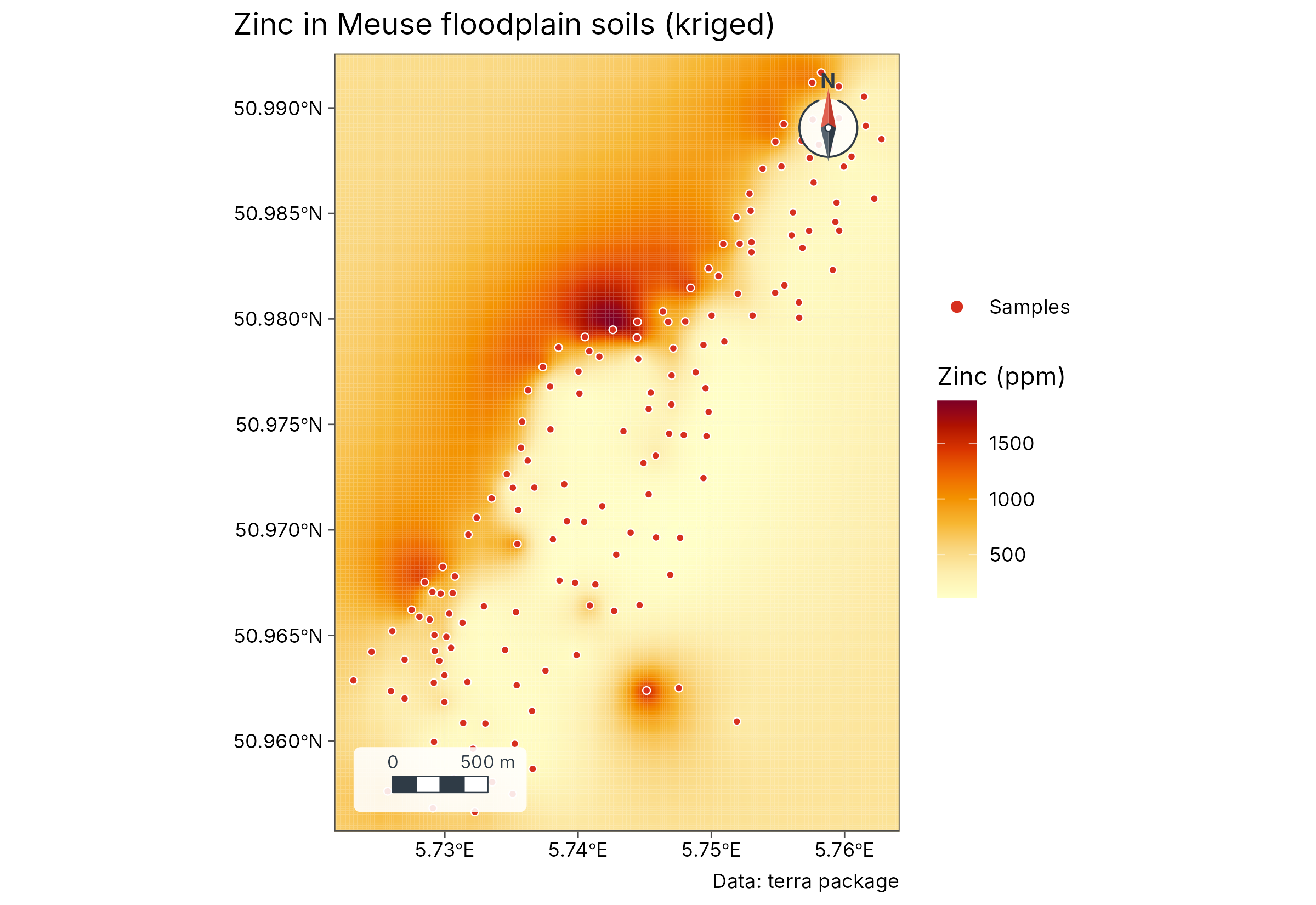
GeoSpaX recipes
The same analysis as a GeoSpaX recipe, run unchanged in R: kriging against IDW by cross-validation, then a map and an HTML report.
rec <- geo_recipe_read(system.file("recipes/interpolate-samples.yaml", package = "tidymapr"))
rec
#> GeoSpaX recipe "interpolate-samples" (v2): Field samples → interpolated surface
#> (kriging or IDW, automatically)
#> Inputs: layer and field
#> Steps: samples (io.open), surface (interpolate.auto), style_samples
#> (automap.style), map (export.map), uncertainty (export.map), and report
#> (export.report)
#> Outputs: surface, map, uncertainty, and report
out <- geo_recipe_run(rec, inputs = list(layer = samples, field = "zinc"), dir = tempfile(), quiet = TRUE)
out$log
#> # A tibble: 6 × 4
#>   step          use              status seconds
#>   <chr>         <chr>            <chr>    <dbl>
#> 1 samples       io.open          done      0
#> 2 surface       interpolate.auto done      5.93
#> 3 style_samples automap.style    done      0
#> 4 map           export.map       done      1.24
#> 5 uncertainty   export.map       done      1.06
#> 6 report        export.report    done      0
Hot spots and clusters
Getis-Ord Gi* and local Moran’s I (LISA) find places of unusually high or low values; both match spdep.
hot <- geo_hotspot(sf::st_transform(samples, 4326), zinc, k = 8)
count(sf::st_drop_geometry(hot), hotspot)
#>           hotspot   n
#> 1             hot  24
#> 2            cold  28
#> 3 not significant 103
geo_map(title = "Hot spots of zinc (Getis-Ord Gi*)", crs = 28992) |>
  map_points(hot, fill = hotspot, group = "Gi*", palette = c("#2166AC", "#B2182B", "grey80"), size = 2)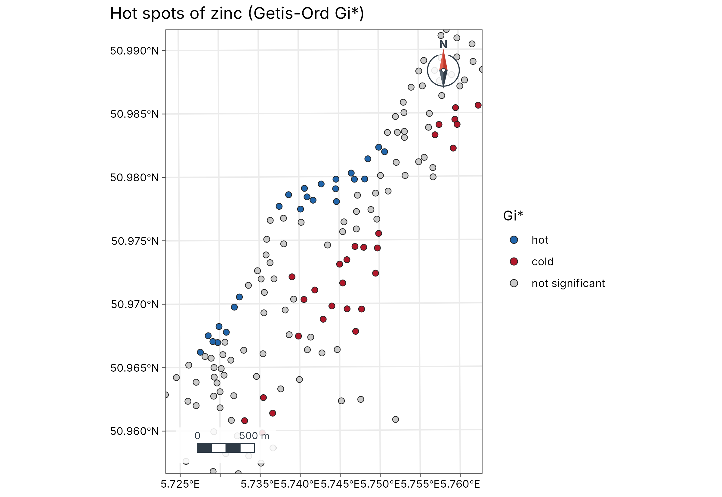
geo_dbscan() groups points into density clusters, here
1,000 earthquakes near Fiji (datasets::quakes), with
distances in metres.
cl <- geo_dbscan(datasets::quakes, eps = 50000, min_pts = 15, lon = long, lat = lat)
table(cl$cluster)
#>
#>   0   1   2   3   4   5   6   7   8   9
#> 513 259  23  25  76  19  26  17  27  15
attr(cl, "hulls")
#> Simple feature collection with 9 features and 2 fields
#> Geometry type: POLYGON
#> Dimension:     XY
#> Bounding box:  xmin: -179.98 ymin: -28.1 xmax: 179.69 ymax: -10.96
#> Geodetic CRS:  WGS 84
#>   cluster   n                       geometry
#> 1       1 259 POLYGON ((-179.36 -22.64, -...
#> 2       2  23 POLYGON ((-175.94 -20.31, -...
#> 3       3  25 POLYGON ((165.76 -12.08, 16...
#> 4       4  76 POLYGON ((-179.98 -25.59, 1...
#> 5       5  19 POLYGON ((-174.68 -16.1, -1...
#> 6       6  26 POLYGON ((169.5 -19.64, 169...
#> 7       7  17 POLYGON ((-173.2 -15.66, -1...
#> 8       8  27 POLYGON ((-177.75 -28.1, -1...
#> 9       9  15 POLYGON ((-175.36 -23.95, -...
Terrain and hydrology
D8 flow direction, flow accumulation, watersheds and the topographic wetness index on Luxembourg’s elevation model; they match terra.
dem <- terra::project(terra::rast(system.file("ex/elev.tif", package = "terra")), "EPSG:2169")
acc <- geo_flow_accumulation(dem)
cantons <- sf::st_read(system.file("ex/lux.shp", package = "terra"), quiet = TRUE)
geo_map(title = "Where water collects: flow accumulation") |>
  map_raster(log10(acc), name = "log10 cells", palette = "Blues 3") |>
  map_polygons(cantons, preset = "admin", label = "Cantons")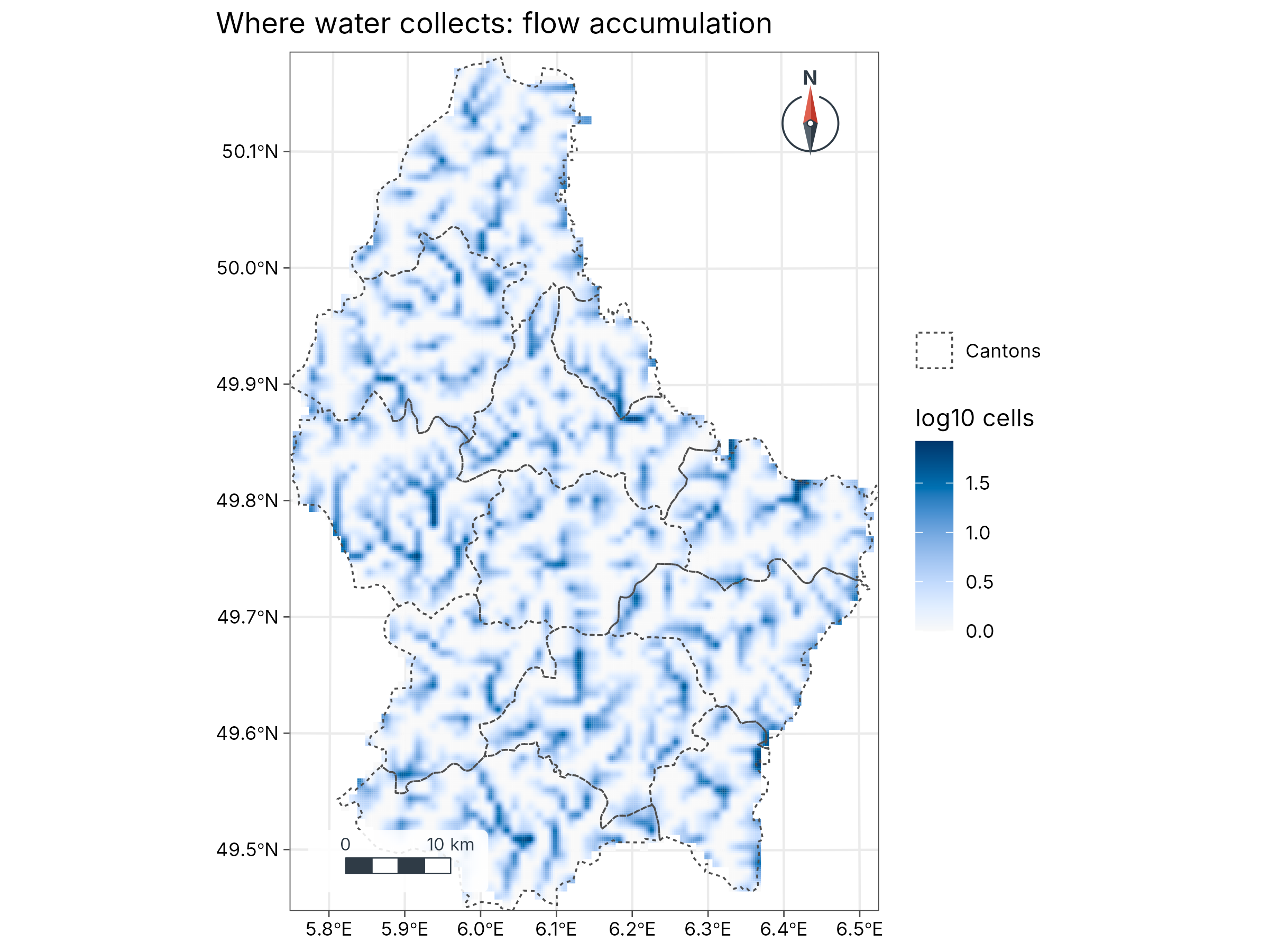
Remote sensing
Spectral indices with an automatic (Otsu) threshold, and spectral diversity in Hill numbers, on a Sentinel-2 scene of Luxembourg.
s2 <- terra::rast(system.file("ex/sent2_L2A_2024-08-24.tif", package = "terra"))
ndvi <- geo_spectral_index(s2, "NDVI")
set.seed(1)
sdiv <- geo_spectral_diversity(s2, window = 5, k = 15)
a <- geo_map(subtitle = "NDVI", north_arrow = FALSE) |>
  map_raster(ndvi, name = "NDVI", palette = "Greens 3")
b <- geo_map(subtitle = "Spectral diversity (q = 1)", scale_bar = FALSE) |>
  map_raster(sdiv[[1]], name = "Effective\nspectral species", palette = "viridis")
geo_panels(a, b, ncol = 2, guides = "keep")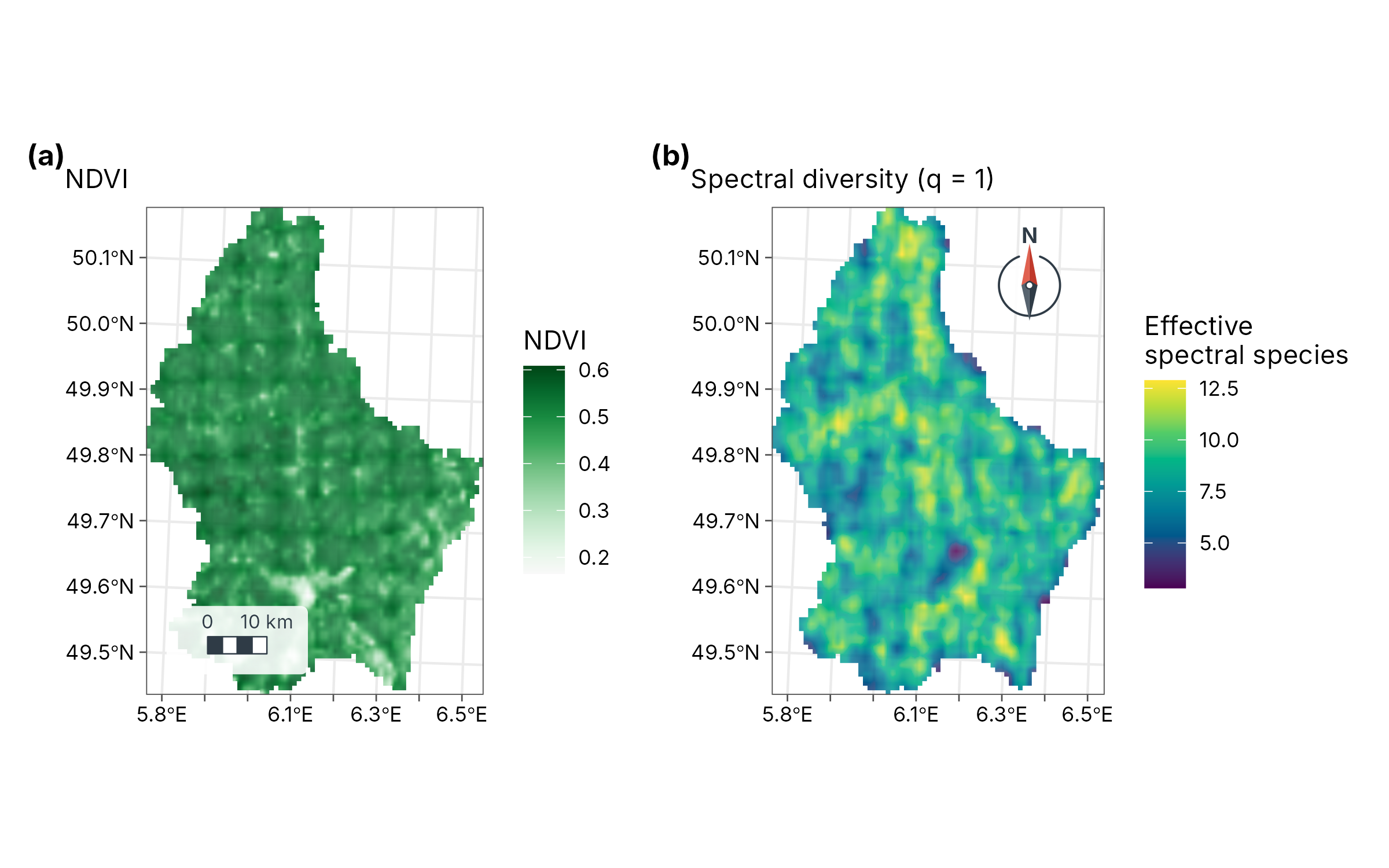
Fresh imagery comes from STAC catalogues; only the window over the area is downloaded:
city <- c(6.08, 49.57, 6.18, 49.65)
scenes <- geo_stac_search("sentinel-2-l2a", city,
  datetime = c("2024-06-01", "2024-08-31"), cloud_cover = 10
)
img <- geo_stac_read(scenes, c("red", "nir"), area = city, n = 4)
geo_spectral_index(img, "NDVI")
Landscape fragmentation
FRAGSTATS metrics per land-cover class; they match landscapemetrics on projected rasters and are measured in true hectares on rasters in degrees.
e <- new.env()
utils::data("augusta_nlcd", package = "landscapemetrics", envir = e)
lc <- e$augusta_nlcd
if (inherits(lc, "PackedSpatRaster")) lc <- terra::unwrap(lc)
geo_landscape(lc) |> arrange(desc(ca)) |> head(6)
#> # A tibble: 6 × 9
#>   class    np    ca pland    lpi area_mn    ed    ai   mesh
#>   <dbl> <int> <dbl> <dbl>  <dbl>   <dbl> <dbl> <dbl>  <dbl>
#> 1    42  1795 9991. 37.2  1.61     5.57   95.2  80.9 41.6
#> 2    41  1880 5036. 18.8  1.27     2.68   72.3  71.2  9.85
#> 3    81   828 2281.  8.49 0.373    2.75   29.7  74.1  1.94
#> 4    43  2402 2133.  7.94 0.0825   0.888  55.9  47.3  0.225
#> 5    71  1300 1693.  6.31 0.306    1.30   26.8  68.5  1.01
#> 6    21  3757 1398.  5.21 0.0801   0.372  44.2  36.4  0.150
geo_landscape(lc, "landscape")
#> # A tibble: 1 × 6
#>      np     ta    ed  shdi  sidi  mesh
#>   <int>  <dbl> <dbl> <dbl> <dbl> <dbl>
#> 1 17141 26849.  204.  1.99 0.801  59.6
Species distribution models
sdm_maxent() fits Maxent in C++ and
sdm_ensemble() combines it with a GLM, a GAM and a random
forest under spatial cross-validation. See the sloth case study for a complete
example.