5. Species distribution models: Maxent and ensembles

The concept

A species distribution model (SDM) relates where a species has been recorded to the environment there, then predicts how suitable every other place is. It rests on the ecological niche (Hutchinson 1957): the set of environmental conditions in which a species can persist. The model learns the niche in environmental space (temperature, rainfall, …) and projects it back into geographic space as a map.

Most records are presence-only: museum specimens, GBIF occurrences, camera-trap sightings. Absences are rarely recorded, and a missing record does not mean the species is absent. So the model compares presences with background points, a random sample of the environments available in the study region. It asks: how do the conditions at presences differ from the conditions available?

library(tidymapr)
library(dplyr)

The data

116 records of the brown-throated sloth, Bradypus variegatus, and WorldClim bioclimatic variables, from the original Maxent paper (Phillips et al. 2006), shipped with the predicts package.

occ <- read.csv(system.file("ex/bradypus.csv", package = "predicts"))
climate <- terra::rast(system.file("ex/bio.tif", package = "predicts"))
climate <- climate[[c("bio1", "bio5", "bio6", "bio7", "bio8", "bio12", "bio16", "bio17")]]
climate <- terra::crop(climate, terra::ext(-95, -32, -35, 22))

set.seed(1)
bg <- suppressWarnings(terra::spatSample(climate, 10000, "random", na.rm = TRUE, xy = TRUE))
pv <- terra::extract(climate, occ[, c("lon", "lat")], ID = FALSE)

d <- rbind(pv, bg[names(climate)])                       # environment at every point
xy <- rbind(as.matrix(occ[, c("lon", "lat")]), as.matrix(bg[, c("x", "y")]))
presence <- c(rep(1, nrow(pv)), rep(0, nrow(bg)))         # 1 = record, 0 = background
ok <- stats::complete.cases(d)
d <- d[ok, ]; xy <- xy[ok, ]; presence <- presence[ok]
table(presence)
#> presence
#>    0    1 
#> 6240  116

Variable	Meaning (WorldClim)	Units
bio1	Annual mean temperature	°C × 10
bio5	Maximum temperature of the warmest month	°C × 10
bio6	Minimum temperature of the coldest month	°C × 10
bio7	Temperature annual range (bio5 − bio6)	°C × 10
bio8	Mean temperature of the wettest quarter	°C × 10
bio12	Annual precipitation	mm
bio16	Precipitation of the wettest quarter	mm
bio17	Precipitation of the driest quarter	mm

1. Maxent

Theory

Maxent (Phillips et al. 2006) estimates the probability distribution of presences over the background cells that has maximum entropy (is as spread out, as uninformative, as possible) subject to one constraint: the average of each environmental feature over the predicted distribution must match its average at the presences. “Assume nothing beyond what the data show.”

This is mathematically the same as a Poisson point process model of presence intensity, and as an infinitely weighted logistic regression of presences against background (Fithian and Hastie 2013; Renner and Warton 2013). tidymapr fits it that way, as maxnet does (Phillips et al. 2017), with the lasso penalty, which shrinks unimportant features to exactly zero.

Features let the model learn non-linear responses:

Class	Code	Shape it can learn	Example
Linear	l	Steadily increasing or decreasing	More suitable where wetter
Quadratic	q	A peak (an optimum)	Suitable at intermediate temperature
Product	p	An interaction between two variables	Heat tolerated only where wet
Hinge	h	A threshold, then a slope	Unsuitable below 1,000 mm, then rising

Regularisation (regmult, default 1) sets how strongly the lasso penalises complexity. Larger values give smoother, more general models; smaller values fit the training data more closely and risk overfitting.

mx <- sdm_maxent(presence, d)
mx
#> Maxent (lqph features, regmult 1): 116 presences, 6240 background points,
#> standardised predictors, 28 non-zero features of 820.
#> Features kept: linear 6, quadratic 3, product 5, hinge 14.

Interpretation. Of 820 candidate features, the lasso kept 28. The rest were not needed to describe how presences differ from the background.

Why tidymapr standardises predictors

Quadratic and product features depend on where zero lies. maxnet, the R port of Maxent, builds them from the raw values, so the same climate in different units gives a different model. tidymapr rescales every predictor to 0-1 first, as the original Java Maxent does, so results do not depend on units. A test: express temperature in tenths of a kelvin instead of tenths of a degree Celsius.

temp <- c("bio1", "bio5", "bio6", "bio8")
d_kelvin <- d
d_kelvin[temp] <- d_kelvin[temp] + 2731.5   # tenths of °C -> tenths of K

change <- function(standardize) {
  a <- sdm_maxent(presence, d, standardize = standardize)
  b <- sdm_maxent(presence, d_kelvin, standardize = standardize)
  max(abs(predict(a, d) - predict(b, d_kelvin)))
}
knitr::kable(tibble(
  model = c("Raw predictors (as maxnet)", "Standardised (tidymapr default)"),
  `largest change in suitability` = c(change(FALSE), change(TRUE))
), digits = 4, caption = "Changing temperature units from Celsius to kelvin: how much does predicted suitability (0-1) change?")

Changing temperature units from Celsius to kelvin: how much does predicted suitability (0-1) change?

model	largest change in suitability
Raw predictors (as maxnet)	0.2065
Standardised (tidymapr default)	0.0000

The climate is identical in both cases; only the units differ. A scientific result should not depend on that, and with standardisation it does not.

Response curves: what the model learned

A response curve shows how predicted suitability changes along one variable while the others are held at their median. It is how you explain an SDM: it describes the niche.

curve <- function(var, label, scale = 1) {
  grid <- as.data.frame(lapply(d, function(x) rep(median(x), 100)))
  grid[[var]] <- seq(min(d[[var]]), max(d[[var]]), length.out = 100)
  tibble(value = grid[[var]] / scale, suitability = predict(mx, grid), variable = label)
}
rc <- bind_rows(
  curve("bio1", "Annual mean temperature (°C)", scale = 10),
  curve("bio12", "Annual precipitation (mm)")
)
ggplot2::ggplot(rc, ggplot2::aes(value, suitability)) +
  ggplot2::geom_line(colour = "#349295", linewidth = 1) +
  ggplot2::facet_wrap(~variable, scales = "free_x") +
  ggplot2::labs(x = NULL, y = "Predicted suitability (cloglog)") +
  theme_tidymapr()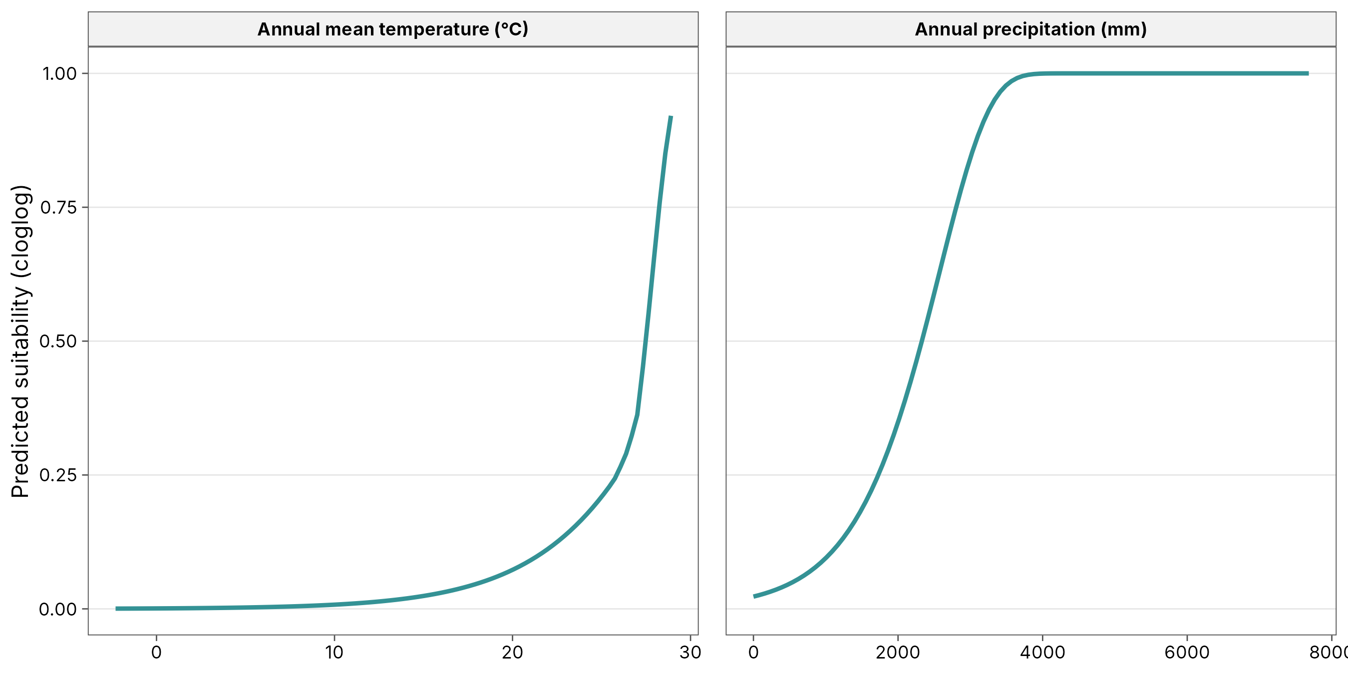

Interpretation. Read each curve as “other things being equal”. Where the curve is high, conditions are like those at the records; where it is low, they are not. A curve that rises to the edge of the data means the optimum may lie outside the study region: be careful predicting there.

2. Evaluation: how good is the model?

Spatial block cross-validation

Testing a model on random held-out points flatters it: test points sit next to training points and share their conditions (Chapter 3: autocorrelation). Spatial block cross-validation (Roberts et al. 2017) holds out whole regions instead, so the model is tested on places it has not seen. sdm_ensemble() splits the region into blocks, groups them into folds balanced for presences and background, and fits each algorithm k times.

Metrics

Metric	What it measures	Range	Rough guide
AUC (area under the ROC curve)	Probability that a random presence gets a higher prediction than a random background point	0.5 = random, 1 = perfect	> 0.7 useful, > 0.8 good. Presence-background AUC cannot reach 1, because background points may be suitable
TSS (true skill statistic)	Sensitivity + specificity − 1, at the best threshold	−1 to 1; 0 = random	> 0.4 useful, > 0.6 good
Boyce index (continuous)	Do presences fall more often than expected in cells predicted as suitable? A rank correlation	−1 to 1; 0 = random	> 0.5 good. The best metric for presence-only data (Hirzel et al. 2006)

3. Ensembles

Theory

Different algorithms make different assumptions, and no single algorithm is best for every species (Elith et al. 2006). An ensemble averages several, weighted by how well each predicted held-out regions, which reduces the risk of relying on one algorithm’s quirks (Araújo and New 2007). tidymapr combines:

Algorithm	Type	Strength
Maxent	Penalised point-process model	Designed for presence-background data; smooth responses
GLM	Logistic regression with quadratic terms	Simple, interpretable optima
GAM	Logistic regression with smooth splines	Flexible curves, still smooth
Random forest (C++)	Many decision trees	Captures interactions and thresholds automatically

ens <- sdm_ensemble(presence, d, coords = xy, folds = 5, ntree = 500, seed = 1)
knitr::kable(ens$summary, digits = 3, caption = "Spatial block cross-validation of each algorithm, and its weight in the ensemble.")

Spatial block cross-validation of each algorithm, and its weight in the ensemble.

algorithm	auc	tss	boyce	weight
maxent	0.779	0.532	0.307	0.241
glm	0.769	0.507	0.499	0.215
gam	0.784	0.529	0.589	0.238
rf	0.804	0.595	0.629	0.306

Interpretation. Each row is one algorithm tested on regions it did not see. The best AUC here is 0.8 and the best TSS 0.59: useful models, as expected for a wide-ranging species. Weights come from cross-validated TSS, so the better algorithms count more; algorithms below min_tss would be left out.

Suitability and disagreement

suit <- predict(ens, climate, what = "all")
world <- sf::st_read(system.file("shapes/world.gpkg", package = "spData"), quiet = TRUE)
americas <- suppressWarnings(sf::st_crop(world, c(xmin = -95, ymin = -35, xmax = -32, ymax = 22)))
records <- sf::st_as_sf(occ, coords = c("lon", "lat"), crs = 4326)

a <- geo_map(subtitle = "Ensemble suitability", crs = "laea", north_arrow = FALSE) |>
  map_raster(suit[["mean"]], name = "Suitability", palette = "YlGnBu", limits = c(0, 1)) |>
  map_polygons(americas, fill = NA, border = "grey40", linewidth = 0.15, label = "Countries") |>
  map_points(records, preset = "sample_site", label = "Records", size = 1)
b <- geo_map(subtitle = "Disagreement between algorithms (SD)", crs = "laea", scale_bar = FALSE) |>
  map_raster(suit[["sd"]], name = "SD", palette = "Oranges") |>
  map_polygons(americas, fill = NA, border = "grey40", linewidth = 0.15, label = "Countries")
geo_panels(a, b, ncol = 2, guides = "keep")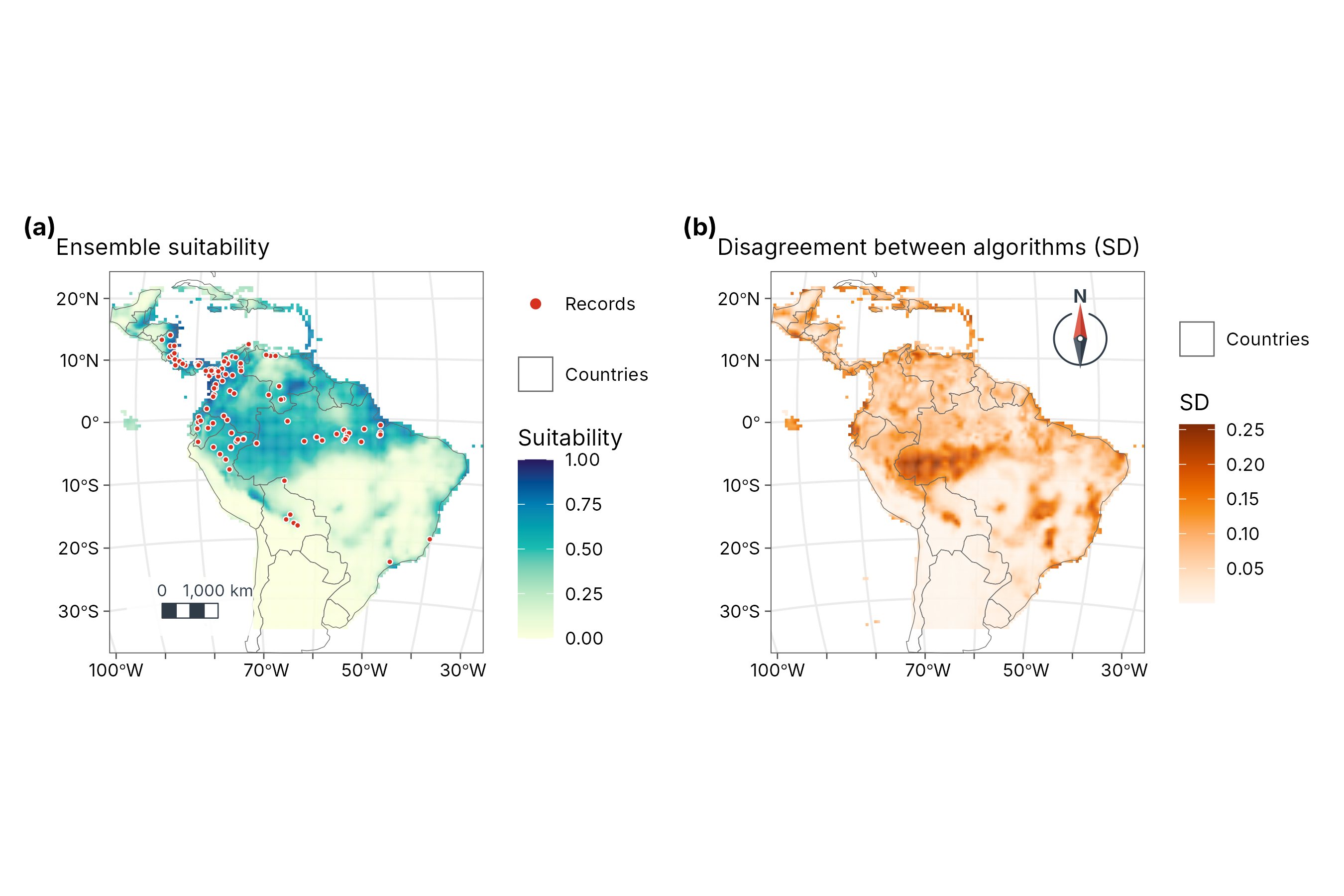

How to read the two maps.

• Suitability (left) is the weighted mean of the four algorithms, from 0 (conditions unlike any record) to 1 (conditions like the core of the records). It is a relative index of environmental similarity, not the probability that the species is present: that would need data on prevalence, which presence-only records do not have.
• Disagreement (right) is the weighted standard deviation among the algorithms. Pale areas: all four agree, so the suitability is robust. Dark areas: they give different answers, often where conditions differ from anywhere the species was recorded. Treat suitability there as uncertain and a priority for field checks.

4. From suitability to a range map: thresholds

Management often needs “suitable / not suitable”. Any cut is a choice:

Threshold	Rule	Effect
Minimum training presence	Lowest suitability at any record	Includes every record; generous range
10th percentile training presence	Excludes the 10 % least suitable records	Robust to a few bad records; common default
Max sensitivity + specificity (maxSSS)	Maximises TSS	Balances omission and commission

State the threshold and why you chose it; show the continuous map as well.

Pitfalls to check

Problem	Symptom	Remedy
Sampling bias: records near roads, cities, field stations	Model maps survey effort, not the species	Thin records (geo_rarefy_spatial()), or sample background with the same bias
Extrapolation to new conditions	Strong predictions in climates outside the training range; high disagreement	Restrict projections; check the disagreement map; clamping (on by default in predict())
Correlated predictors	Unstable response curves	Choose fewer, ecologically meaningful variables
Too few records	Weak cross-validation; erratic curves	Use fewer features (features = "lq") or a larger regmult
Bad coordinates	Records in the sea or at country centroids	Clean with geo_clean() before modelling

How to report it

Follow the ODMAP protocol (Zurell et al. 2020). For example:

We modelled the distribution of Bradypus variegatus from 116 presence records and 6240 background points using eight WorldClim variables. We fitted Maxent (linear, quadratic, product and hinge features, regularisation multiplier 1, predictors standardised to 0-1), a GLM, a GAM and a random forest (500 trees) with tidymapr, and combined them in an ensemble weighted by the true skill statistic from five-fold spatial block cross-validation. Cross-validated AUC ranged from 0.77 to 0.8 and TSS from 0.51 to 0.59. We report the weighted mean suitability and the weighted standard deviation among algorithms as a measure of model uncertainty.

References

Araújo, M. B. and New, M. (2007). Ensemble forecasting of species distributions. Trends in Ecology & Evolution, 22, 42-47.

Elith, J. et al. (2006). Novel methods improve prediction of species’ distributions from occurrence data. Ecography, 29, 129-151.

Fithian, W. and Hastie, T. (2013). Finite-sample equivalence in statistical models for presence-only data. Annals of Applied Statistics, 7, 1917-1939.

Hirzel, A. H. et al. (2006). Evaluating the ability of habitat suitability models to predict species presences. Ecological Modelling, 199, 142-152.

Hutchinson, G. E. (1957). Concluding remarks. Cold Spring Harbor Symposia on Quantitative Biology, 22, 415-427.

Phillips, S. J., Anderson, R. P. and Schapire, R. E. (2006). Maximum entropy modeling of species geographic distributions. Ecological Modelling, 190, 231-259.

Phillips, S. J. et al. (2017). Opening the black box: an open-source release of Maxent. Ecography, 40, 887-893.

Renner, I. W. and Warton, D. I. (2013). Equivalence of MAXENT and Poisson point process models for species distribution modeling in ecology. Biometrics, 69, 274-281.

Roberts, D. R. et al. (2017). Cross-validation strategies for data with temporal, spatial, hierarchical, or phylogenetic structure. Ecography, 40, 913-929.

Zurell, D. et al. (2020). A standard protocol for reporting species distribution models. Ecography, 43, 1261-1277.