






Tidy mapping, spatial analysis and publication cartography.
tidymapr makes publication-quality maps and does spatial analysis in R, in the style of a desktop GIS: one call can choose the projection, classification, colour ramps, legends, scale bar and north arrow, and explain each choice. It is compatible with the GeoSpaX desktop GIS, following the same cartographic conventions, reading and writing the same formats and running the same recipes. For ecology, it is the mapping companion to tidydiversity: tidydiversity estimates diversity, tidymapr puts it on a map. Every verb takes a data frame and returns a tibble, an sf table, a SpatRaster or a ggplot.
Maps and cartography
Automatic, explained maps with geo_automap(); choropleth, bubble and layered maps; Equal Earth, Mercator, UTM and other projections; graticules; GeoSpaX-style scale bars, north arrows and legends; topographic and DEM basemaps.
Installation
Install the development version from GitHub:
# install.packages("pak")
pak::pak("jmozez/tidymapr")
The source code lives on GitHub, https://github.com/jmozez/tidymapr, with a mirror on GitLab, https://gitlab.com/jimmy.moses/tidymapr.
sf, terra and the other spatial packages are optional; install the ones you need with install.packages(c("sf", "terra")).
User guide
New to tidymapr, or to spatial analysis? The User guide explains, chapter by chapter, how to install and run tidymapr in RStudio and what every analysis means: the concept and theory, runnable code on real data, figures and tables, how to interpret them and how to report them in a paper.
Example
A layered map in the style of a desktop GIS layout: each layer gets its own legend section with the symbol for its geometry, and the scale bar, north arrow and projection are set for you. Real data shipped with terra:
library(tidymapr)

elev    <- terra::rast(system.file("ex/elev.tif", package = "terra"))
cantons <- sf::st_read(system.file("ex/lux.shp", package = "terra"), quiet = TRUE)
roads   <- sf::st_as_sf(terra::unwrap(
  readRDS(system.file("ex/lux_highways.rds", package = "terra"))
))

geo_map(title = "Luxembourg", caption = "Data: terra package") |>
  map_raster(elev, name = "Elevation (m)", palette = "Terrain 2", hillshade = TRUE) |>
  map_polygons(cantons, fill = NA, label = "Cantons") |>
  map_lines(roads, colour = highway, palette = c("#B2182B", "#F4A582"), group = "Roads") |>
  map_labels(cantons, text = NAME_2)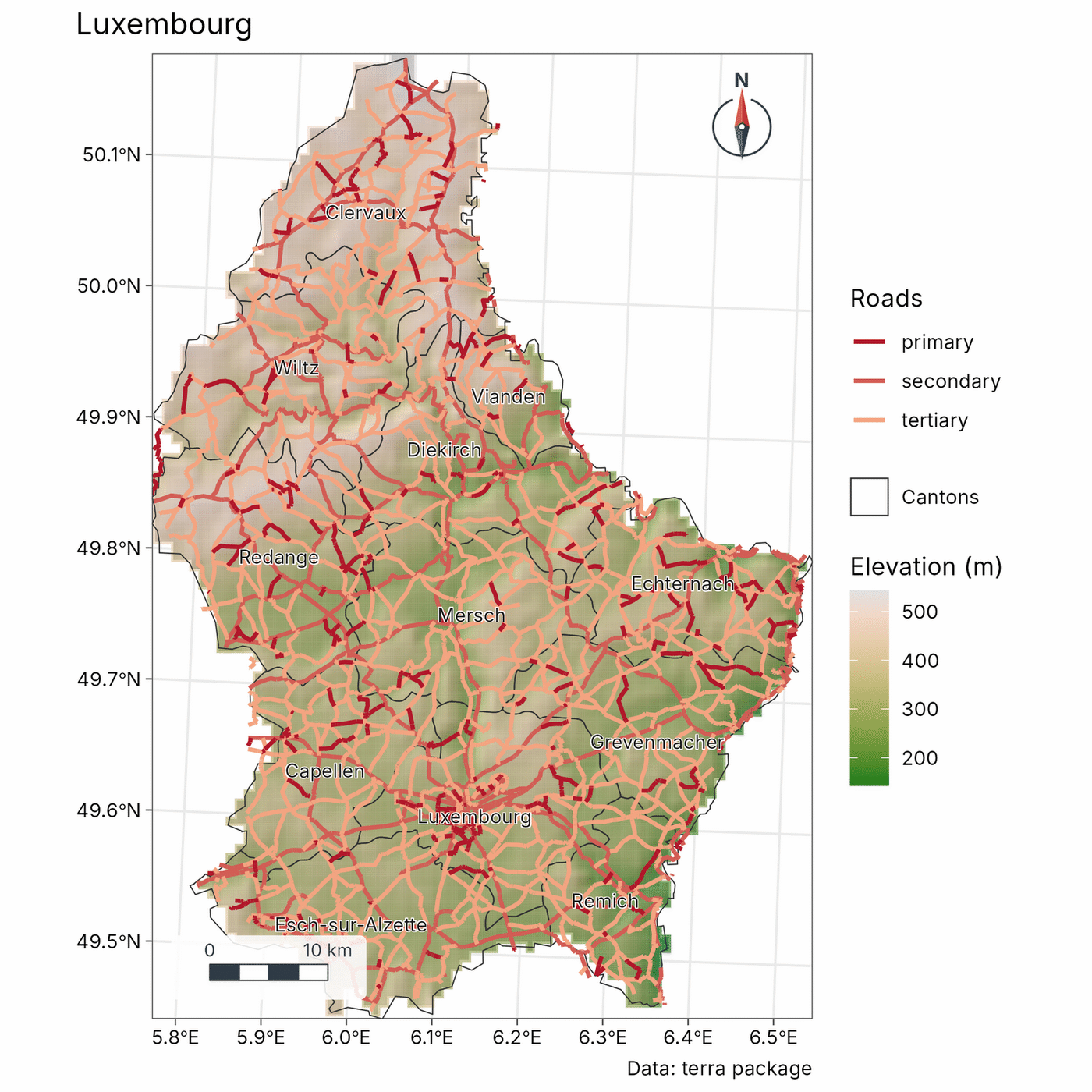
Functions
Gallery
Every map below is made with tidymapr from real, openly licensed data.
Interactive web maps
geo_webmap() turns the same layered map into one interactive HTML page with basemaps, switchable layers, pop-ups and a matching legend.
geo_webmap(m, file = "luxembourg.html")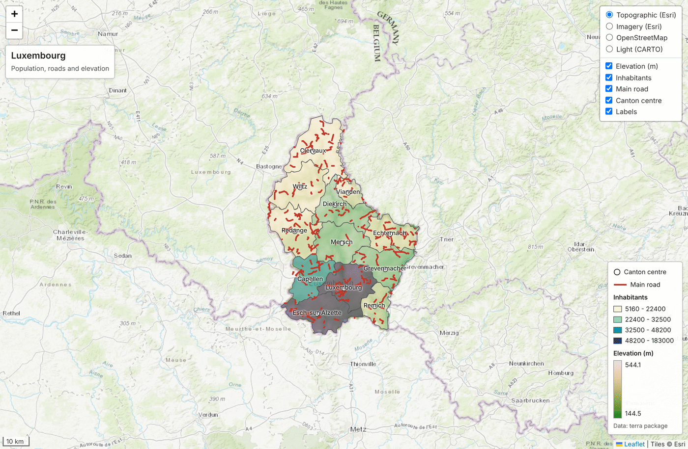
3D terrain maps
geo_map3d() renders a DEM as a lit, shaded 3D block in C++ (no OpenGL), with sites placed on the terrain. Here, the Mt Wilhelm ant survey transect on the Copernicus 30 m DEM, fetched with geo_stac_read().
dem <- geo_stac_search("cop-dem-glo-30", area, cloud_cover = NULL) |>
  geo_stac_read("data", area = area, n = 2)
geo_map3d(dem, theta = 190, phi = 30, points = sites, label = "site")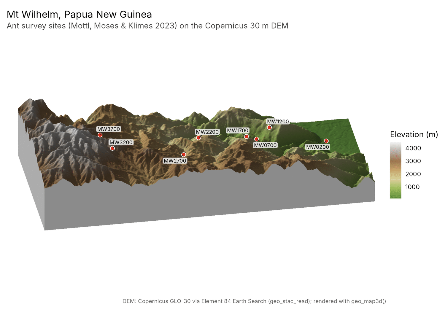
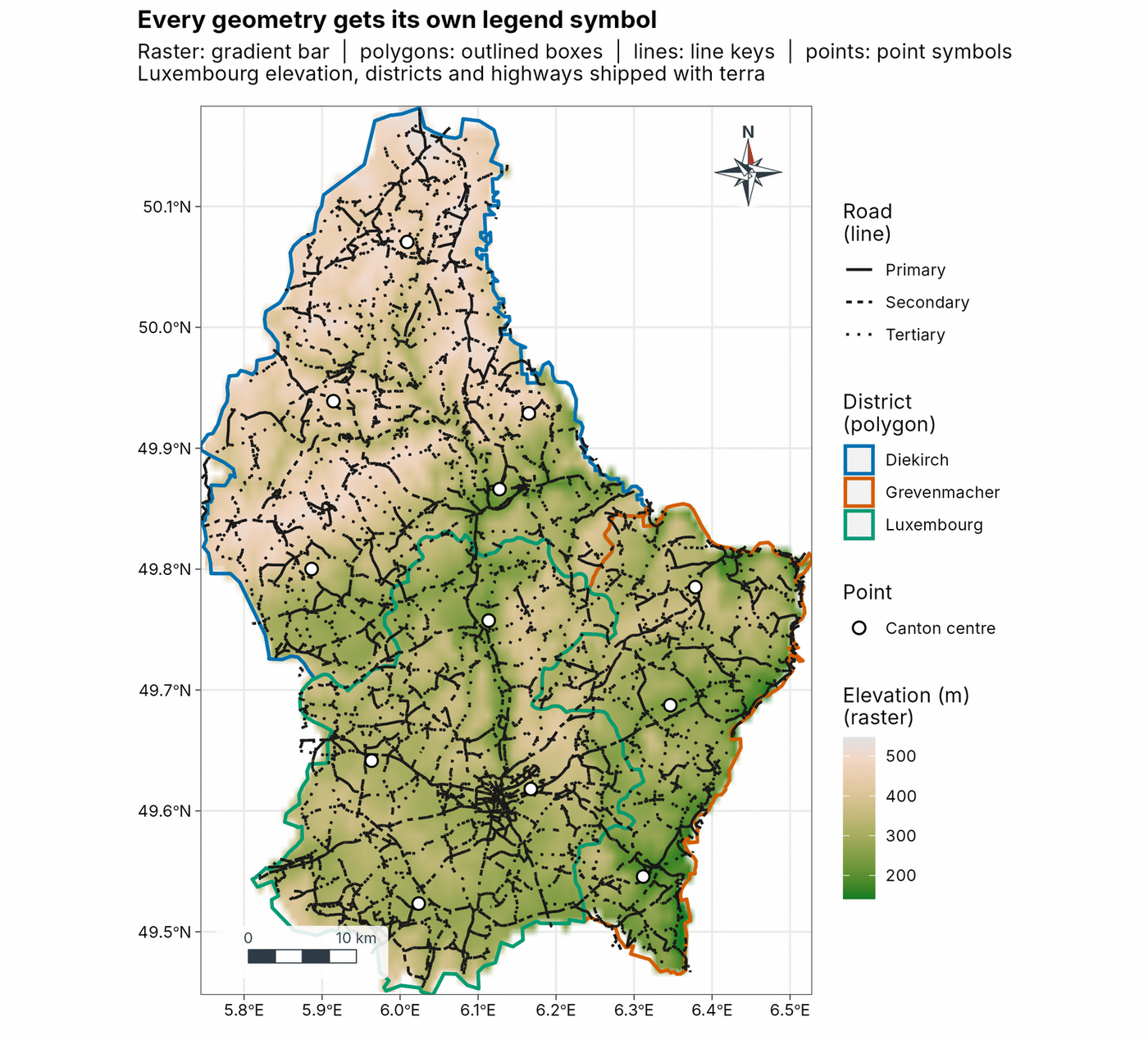
Every geometry gets its own legend symbol
Rasters get a colour bar; polygons, lines and points get swatches, line keys and point symbols, each layer in its own legend section.
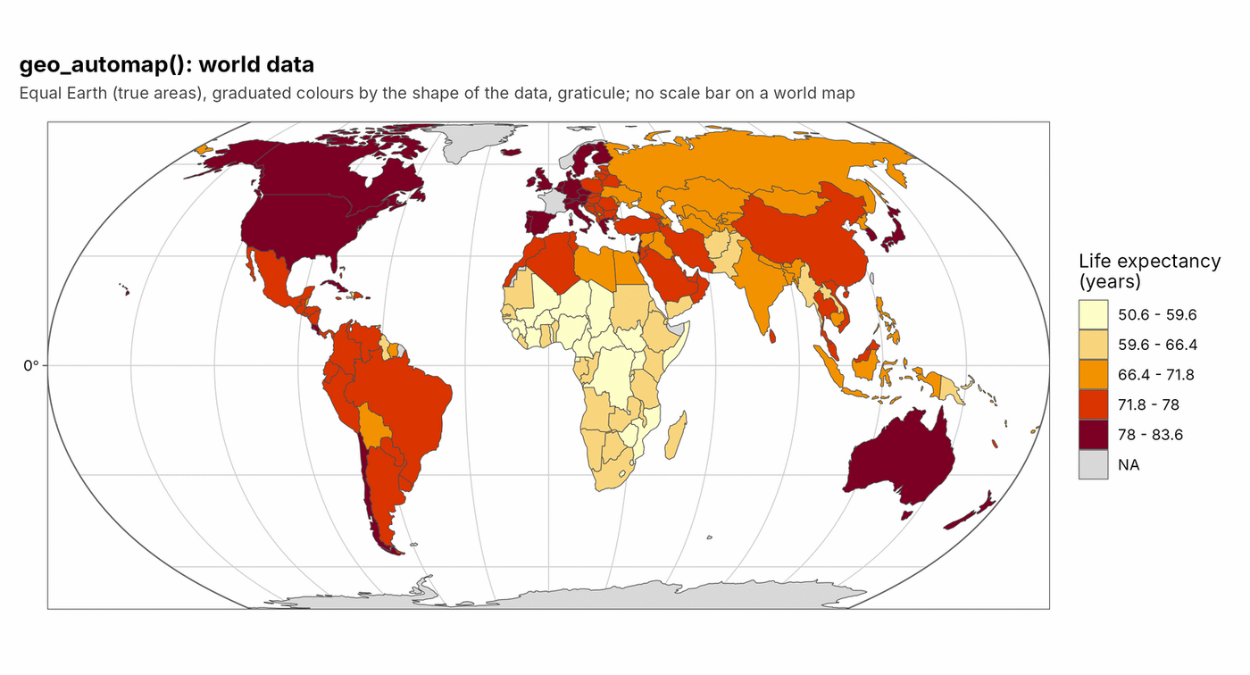
Automatic, explained map design
geo_automap() chooses the projection, classification, colour ramp and map furniture from the data, and geo_automap_explain() says why. Here, world life expectancy on Equal Earth (spData world).
Diversity surfaces with uncertainty
geo_diversity_surface() krigs coverage-standardised Hill numbers with each plot’s estimation error (Barro Colorado Island 50-ha plot, vegan BCI).
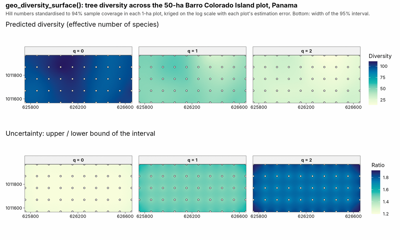
The lower row is the uncertainty: the upper bound of each place’s 95% interval divided by its lower bound. Pale means a precise estimate (a ratio near 1); dark means the true value could lie well above the low end of the range (a ratio of 1.8 means up to 80% higher).
Species distribution ensembles, with Maxent in C++
sdm_maxent() fits Maxent in C++ with the same answers as maxnet (no Java, no glmnet), but standardises predictors first, so results do not depend on units or on where zero lies. sdm_ensemble() combines Maxent, GLM, GAM and a C++ random forest with spatial block cross-validation and TSS weights, and maps where the algorithms disagree.
ens <- sdm_ensemble(presence, climate, coords = xy)
predict(ens, bioclim_raster, what = "all")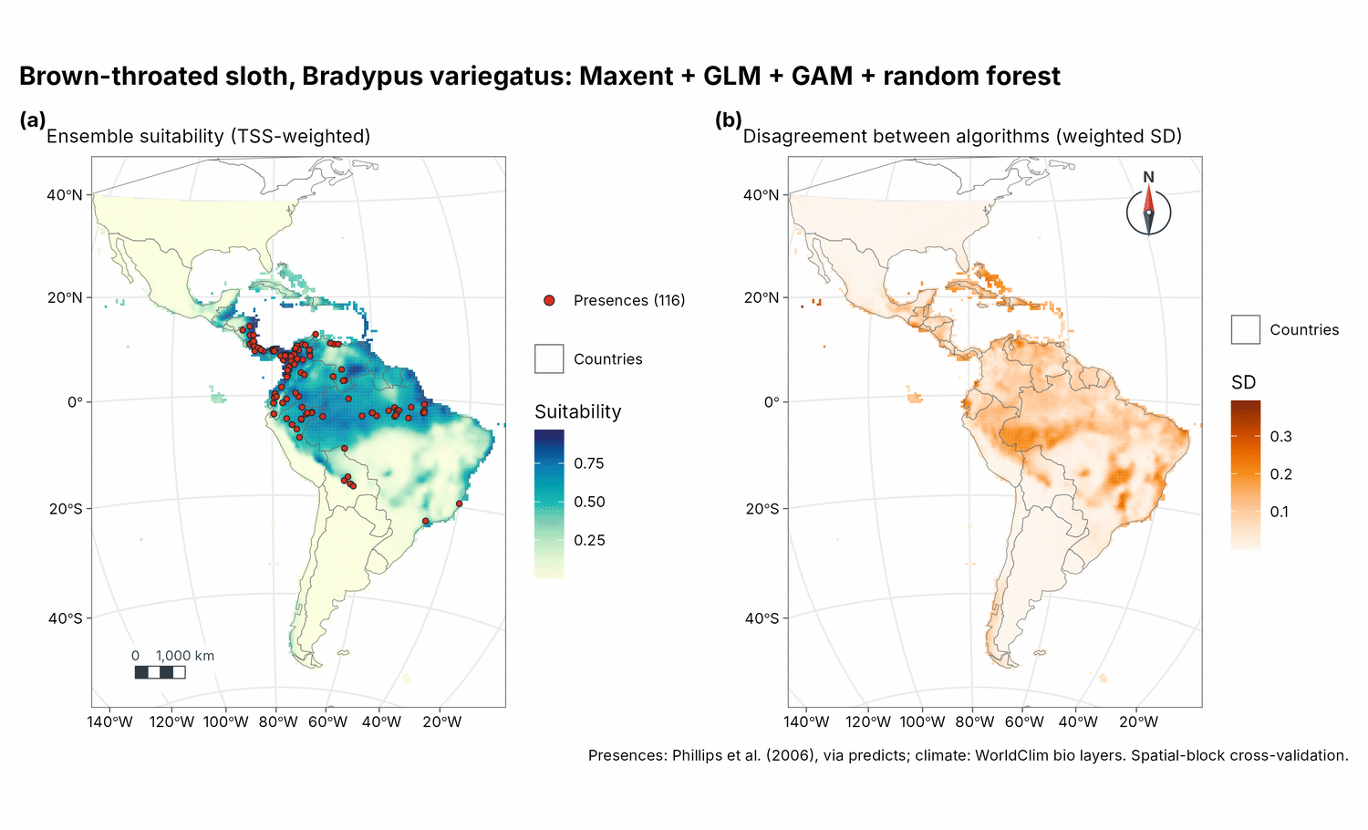
The ensemble map (left) is the weighted average of the four algorithms’ suitability (0 to 1). The disagreement map (right) is how far apart they are at each place (their weighted standard deviation): pale where they agree and the map can be trusted, dark where they give different answers and the prediction is uncertain.
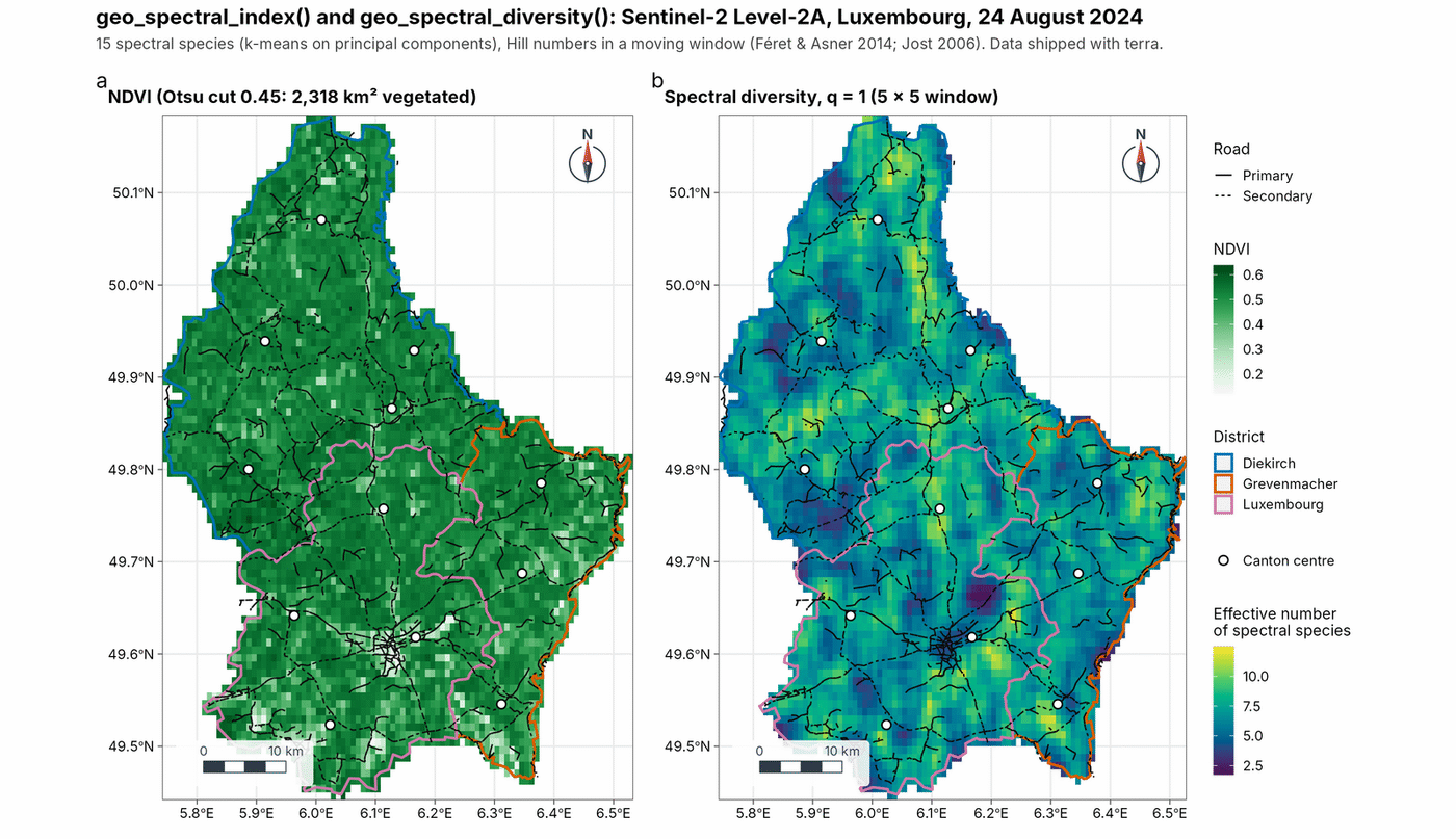
Spectral indices and spectral diversity
NDVI with an Otsu threshold and spectral diversity in Hill numbers from a Sentinel-2 Level-2A scene of Luxembourg (shipped with terra).
Satellite imagery from STAC catalogues
geo_stac_search() and geo_stac_read() find and stream Sentinel-2, Landsat or Copernicus DEM data from STAC catalogues, reading only your area and taking the median of the clearest scenes. Here, NDVI of Luxembourg City in summer 2024.
city   <- c(6.08, 49.57, 6.18, 49.65)
scenes <- geo_stac_search("sentinel-2-l2a", city,
  datetime = c("2024-06-01", "2024-08-31"), cloud_cover = 10)
ndvi   <- geo_stac_read(scenes, c("red", "nir"), area = city, n = 4) |>
  geo_spectral_index("NDVI")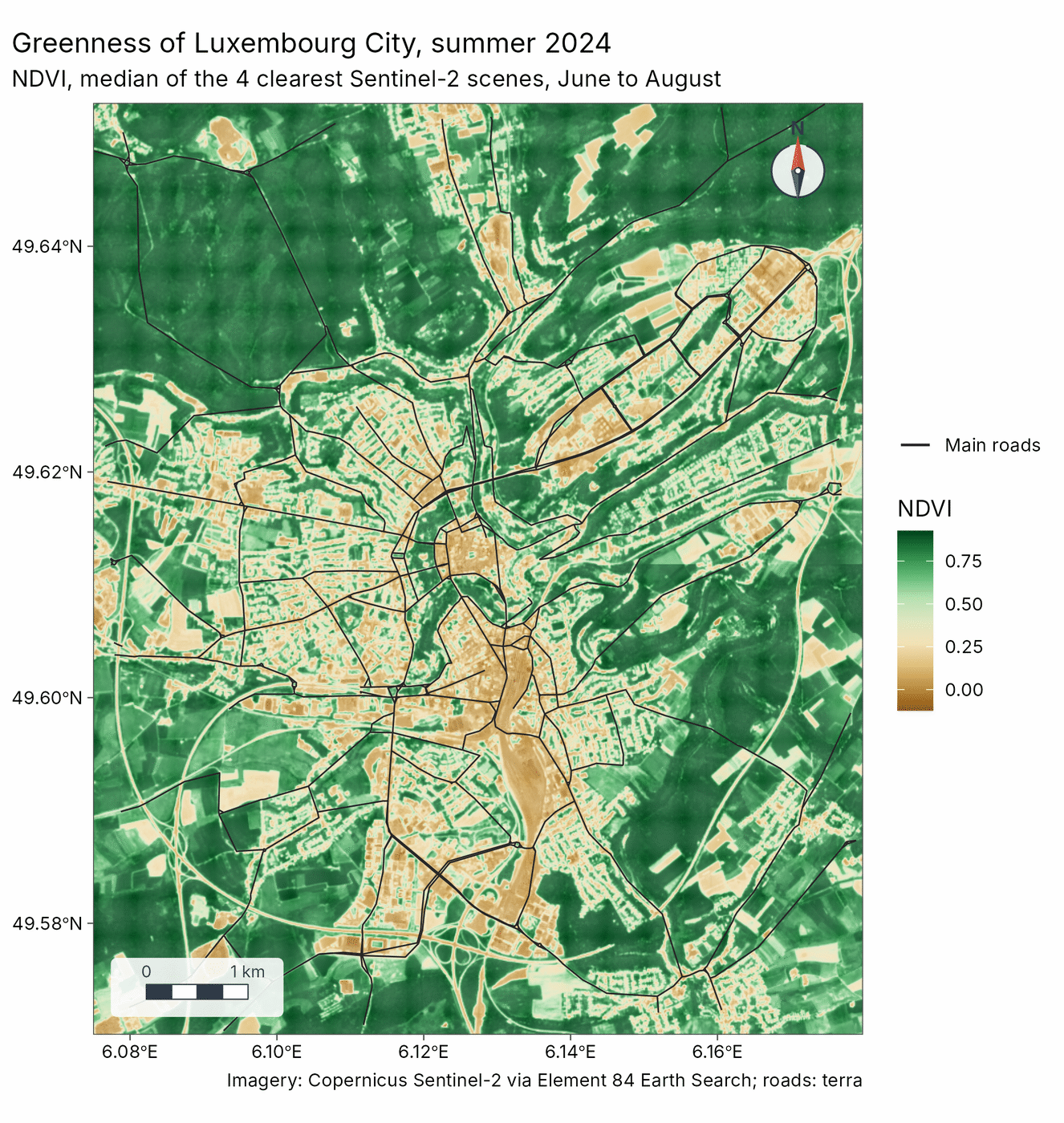
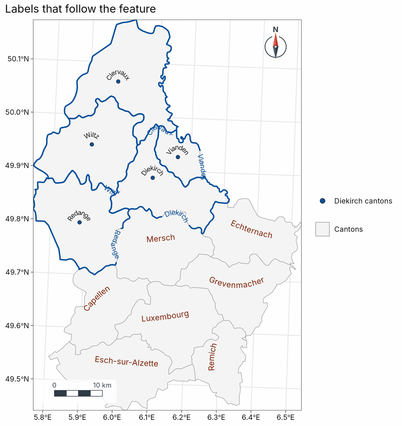
Labels that follow the feature
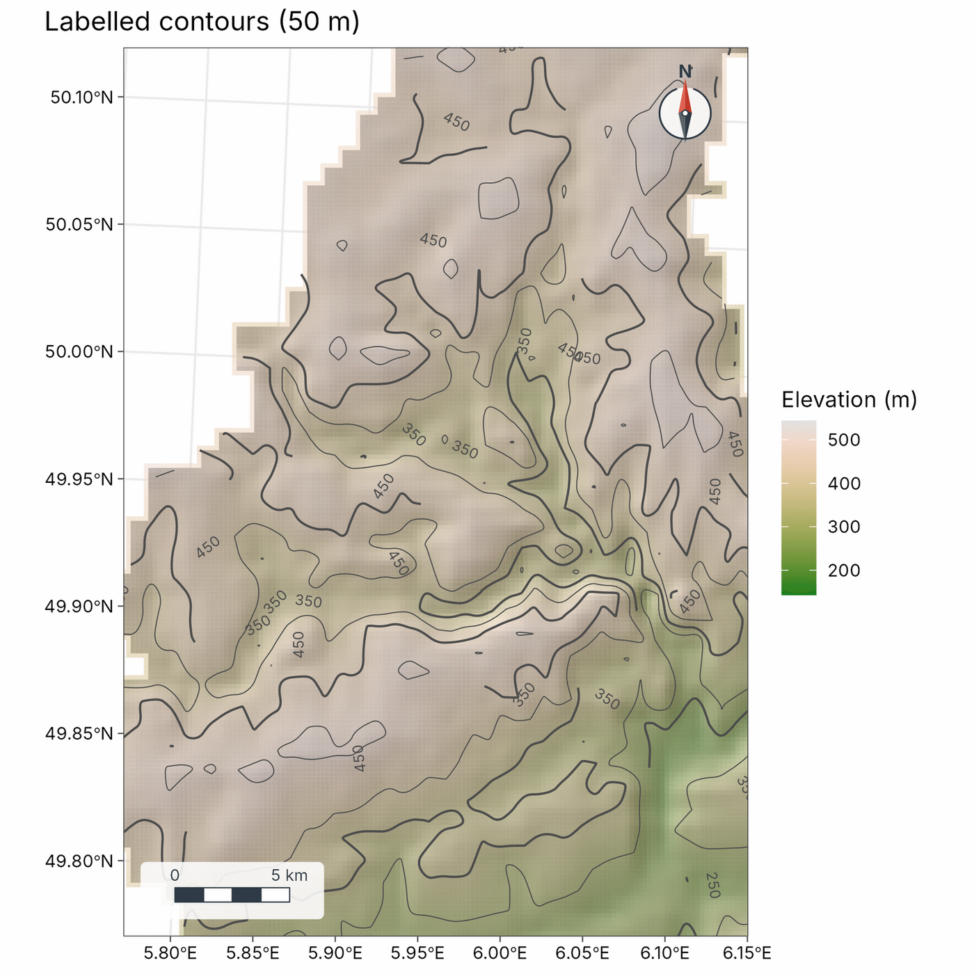
map_curved_labels() writes names along lines, across the long axis or along the outline of polygons, and on an arc above points. map_contours() labels contours at their straightest stretch.
Clusters and fragmentation
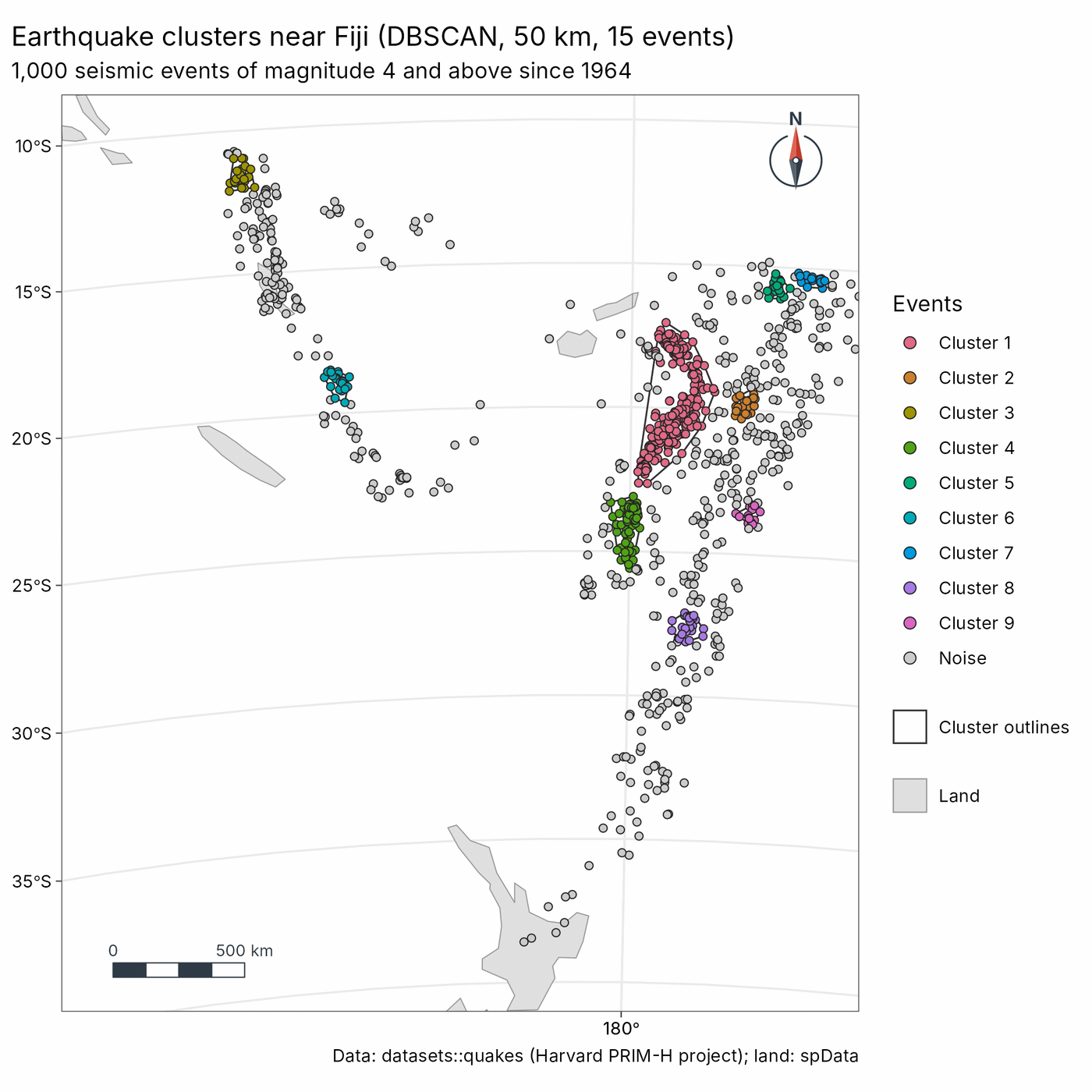
geo_dbscan() finds clusters of points in C++, with distances in metres anywhere on Earth; geo_landscape() measures habitat fragmentation with the FRAGSTATS metrics, matching landscapemetrics and also working on rasters in degrees. Here, earthquake clusters along the Tonga-Kermadec and Vanuatu arcs (datasets::quakes).
Insets, inside legends and small multiples
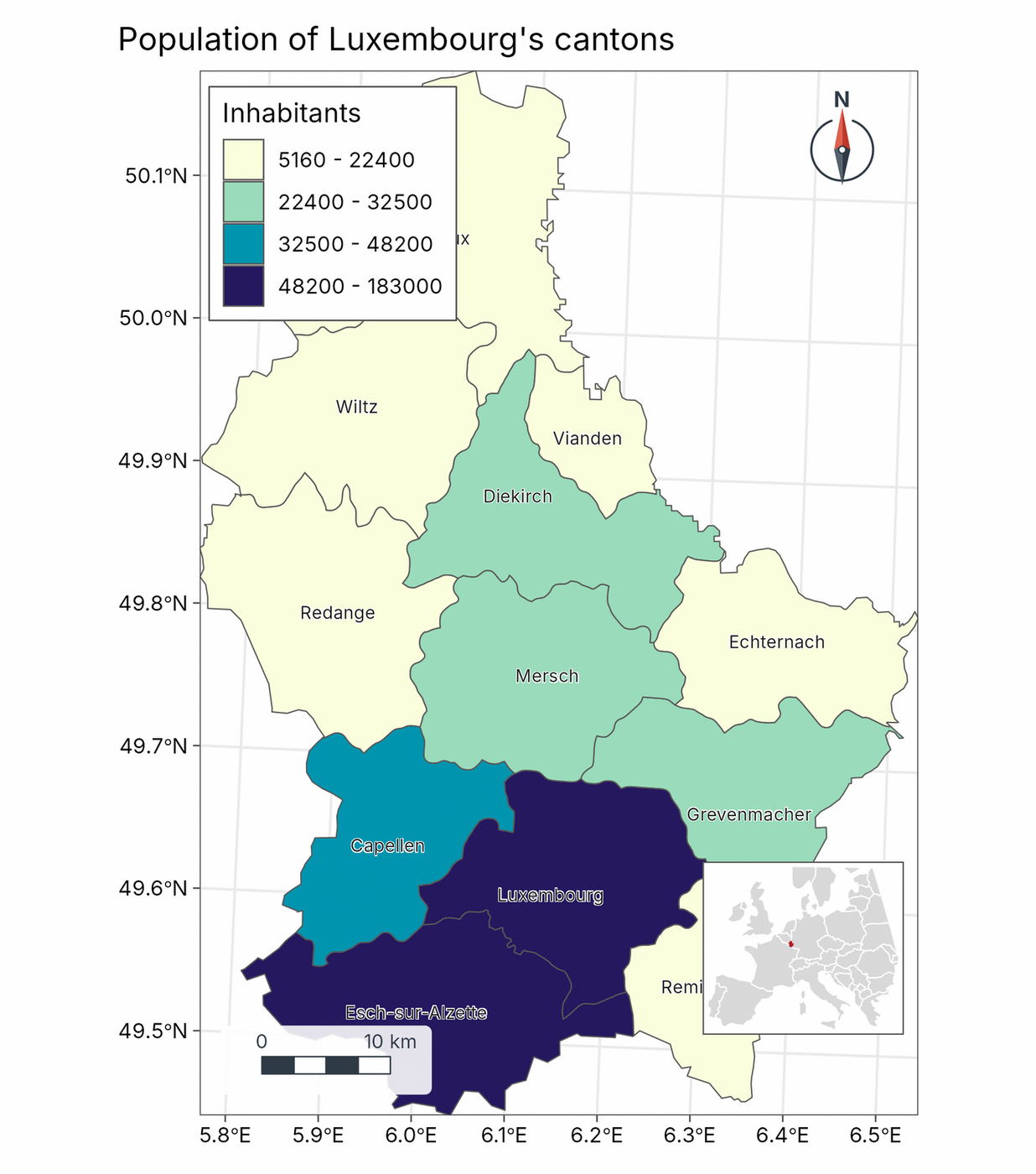
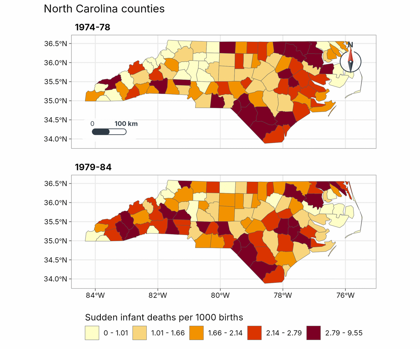
geo_inset() and geo_map(legend = "inside") find corners that do not hide the scale bar, the north arrow or the data. geo_facet_map() draws small multiples with one classification shared by every panel (sudden infant deaths in North Carolina, sf nc).
GeoSpaX recipes in R
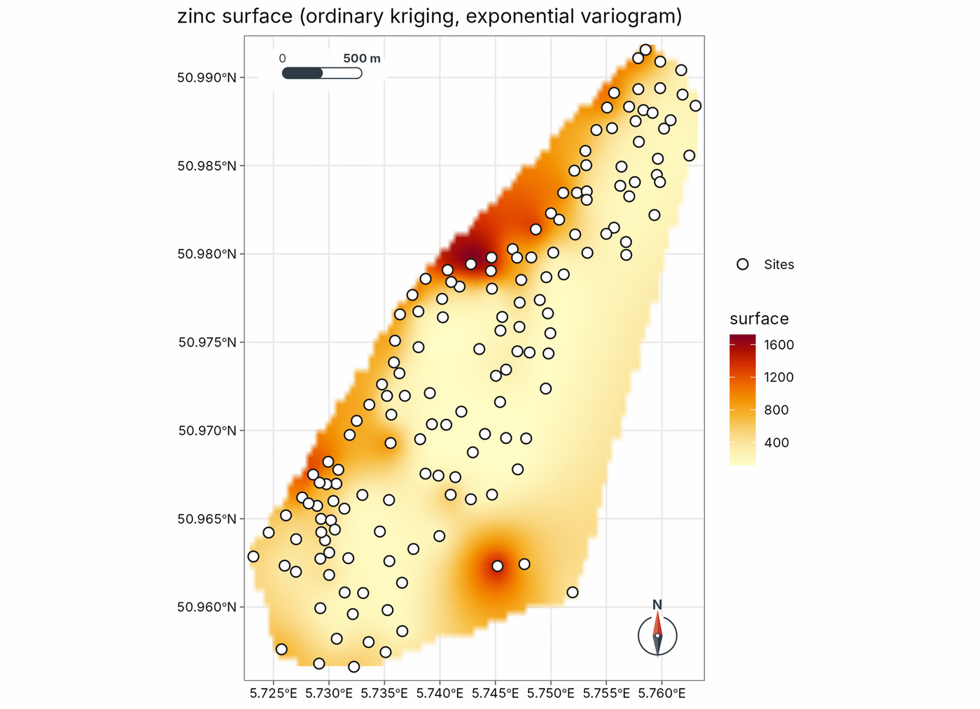
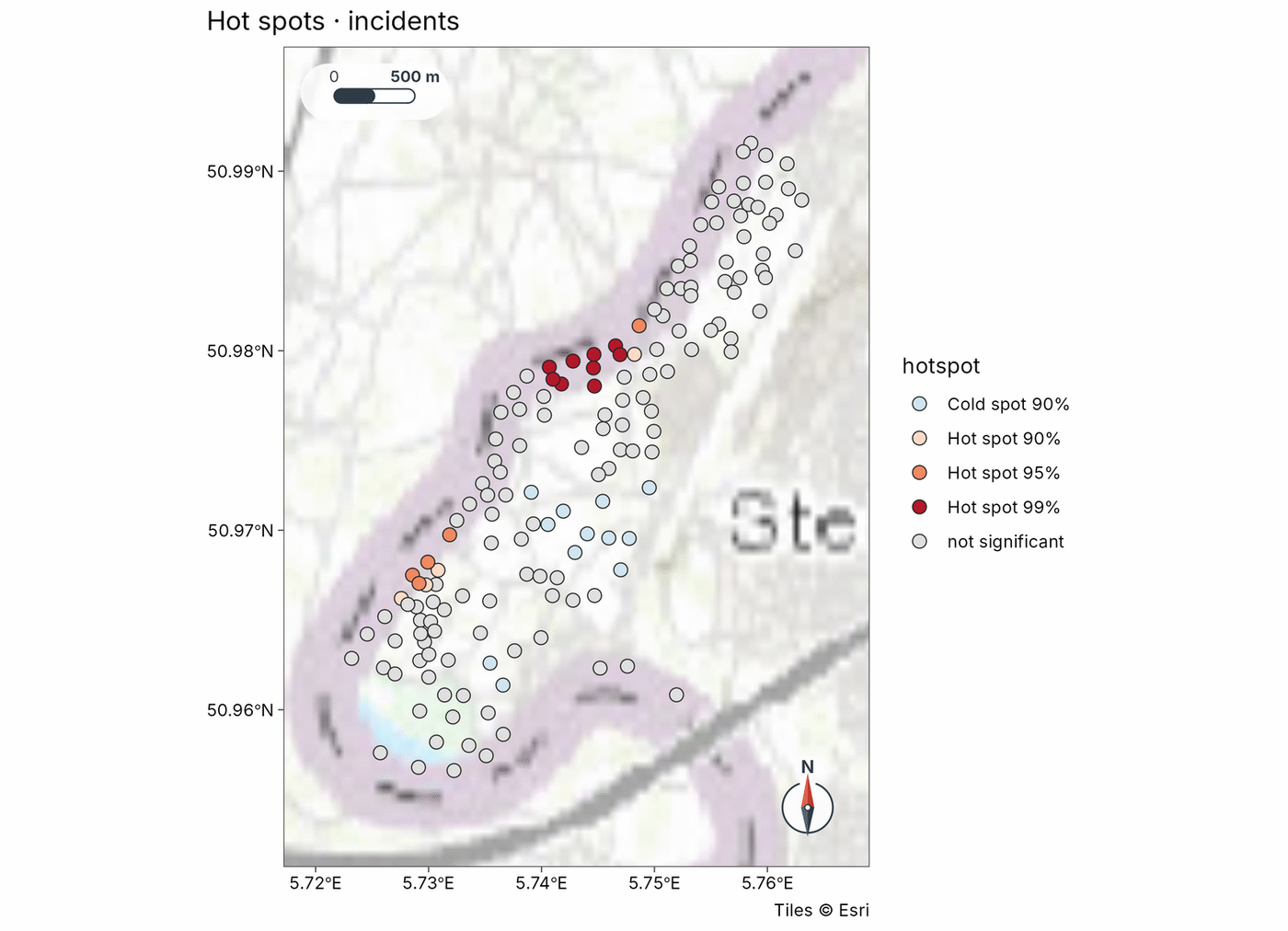
geo_recipe_run() runs GeoSpaX recipes unchanged: kriging against IDW by cross-validation with its standard error, and Getis-Ord hot spots (Meuse soil samples, shipped with terra).
See the gallery for more maps with their code.