Publication-ready study-site maps — plot

plot_sites() draws sampling locations for a manuscript figure: points from an sf table or longitude/latitude columns, optional grouping as colour and shape, non-overlapping labels, an optional raster or coastline backdrop, faceting, a simple scale bar and a north arrow. The result is a ggplot object, so further layers can be added. Diversity values mapped as a continuous fill still use plot_geo(); this verb is for the study-site map that papers usually need first.

The Mt Wilhelm ant data (tidydiversity::png_ants) come with published bait GPS positions in png_ants_sites; geo_example_sites() returns them as one point per elevation band, ready to join by site.

SDM tools such as biomod2 and Maxent are out of scope here; they can be rebuilt later as tidy verbs.

Usage

plot_sites(
  data,
  lon = lon,
  lat = lat,
  colour = NULL,
  shape = NULL,
  label = NULL,
  facet = NULL,
  basemap = "esri",
  raster = NULL,
  coastline = NULL,
  occurrence = NULL,
  size = 3.2,
  occurrence_size = 1.4,
  scale_bar = TRUE,
  north_arrow = TRUE,
  scale_bar_km = NULL,
  scale_units = c("metric", "imperial", "both"),
  palette = c("okabe_ito", "grey"),
  legend_title = NULL,
  legend_position = "auto",
  legend_frame = TRUE,
  inset = FALSE,
  admin = NULL,
  admin_level = 1,
  admin_fill = FALSE
)

Arguments

data: A data frame of sites (or occurrence records) with coordinates, or an sf object.
lon, lat: <data-masking> Coordinate columns when data is not sf.
colour, shape: <data-masking> Optional grouping columns (habitat, elevation band, forest type, season).
label: <data-masking> Optional site labels; overplotting is avoided with ggrepel when installed.
facet: <data-masking> Optional column to facet by (taxon, season).
basemap: Basemap for the figure: "none", "coast", "osm", "carto", "carto_dark", "esri", a SpatRaster, or a file path. See geo_basemap(). Online tiles fall back to "coast" offline.
raster: Optional terra::SpatRaster or file path used as an elevation / climate backdrop (same as passing that object to basemap). Ignored when basemap is not "none".
coastline: Optional sf lines or polygons (for example a country outline) drawn under the sites when using a coast basemap.
occurrence: Optional second data frame of species records with the same coordinate columns, drawn as smaller points underneath the sites.
size: Point size, or a bare column name mapped to point size (combined with colour when both are set, like tmap size + col).
occurrence_size: Point size for occurrence records.
scale_bar, north_arrow: Draw a scale bar and north arrow? TRUE uses the default style, FALSE none, or name a style: scale bars "pill", "checker", "line", "ruler"; north arrows "needle", "compass", "rose", "minimal" (see annotation_scale_bar()).
scale_bar_km: Length of the scale bar in kilometres. When NULL, a round length is chosen from the map extent (true metres via a local UTM projection when the map CRS is geographic).
scale_units: Scale bar units: "metric", "imperial" or "both".
palette: Discrete palette: "okabe_ito" or "grey".
legend_title: Optional legend title (defaults to the colour column).
legend_position: "auto" (collision-aware inside corner), "outside", or a corner "bl" / "br" / "tl" / "tr".
legend_frame: Draw a frame around an inside legend?
inset: Overview / locator map: FALSE, TRUE / "auto", "png" (Papua New Guinea), or a length-4 bbox c(xmin, ymin, xmax, ymax). Placed in a free corner that does not overlap sites, the scale bar, north arrow or inside legend. When GADM data are cached, the PNG inset uses province boundaries from geo_gadm().
admin: Optional administrative boundaries: an sf object (for example from geo_gadm()), or an ISO3 country code that is fetched with geo_gadm(admin, level = admin_level). Drawn as borders, or filled by province when admin_fill is TRUE.
admin_level: GADM level used when admin is a country code (0 country, 1 province, 2 district).
admin_fill: Fill administrative polygons (province choropleth colours) instead of outline-only borders.

Value

A ggplot object. Attribute tmr_decoration holds the reserved corner boxes (for tests and debugging).

Examples

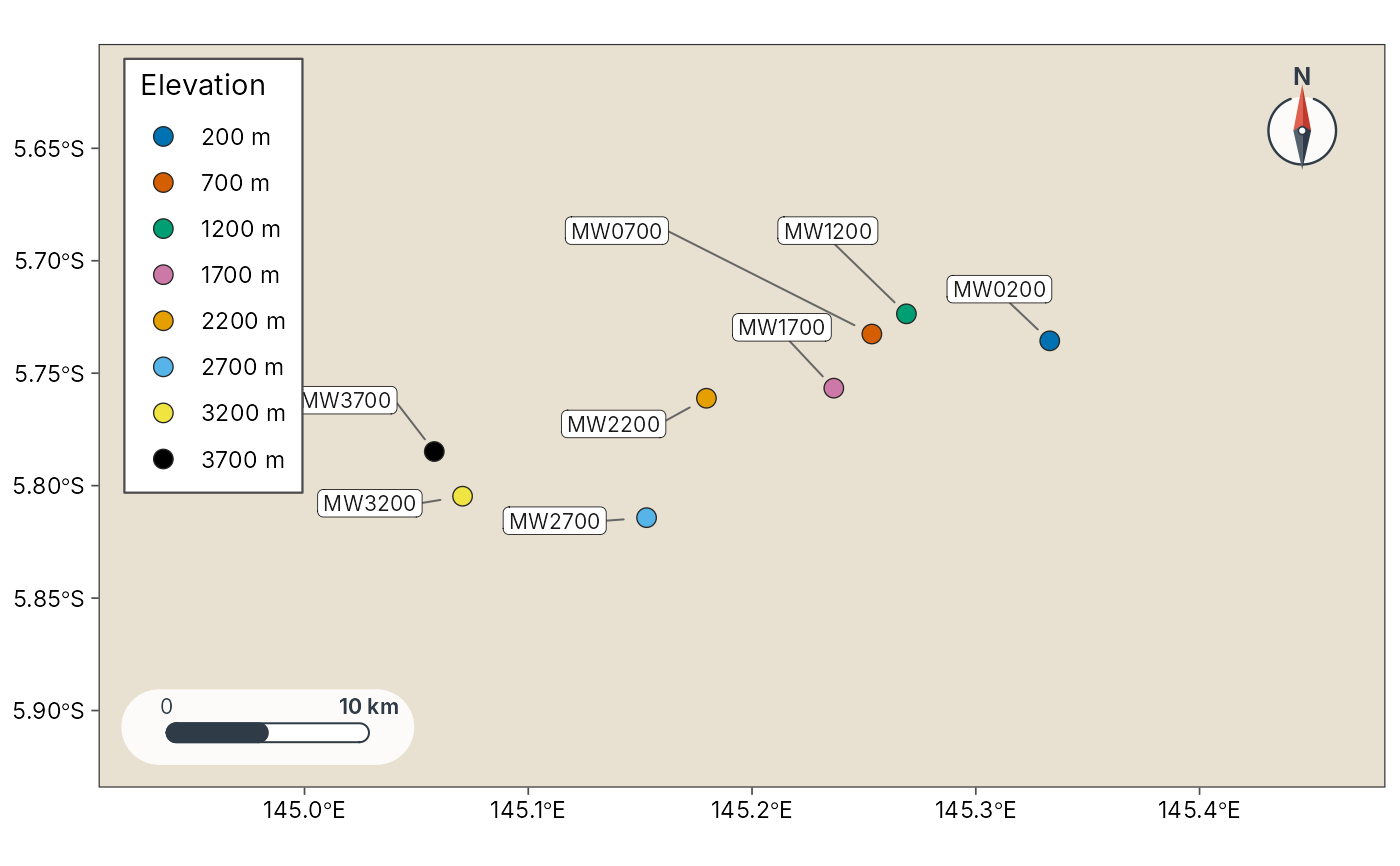
sites <- geo_example_sites("wilhelm")
plot_sites(sites, lon, lat, colour = elevation_band, label = site,
  basemap = "coast")


# Facet by a grouping column
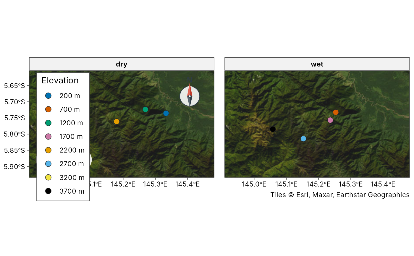
sites$season <- rep(c("dry", "wet"), length.out = nrow(sites))
plot_sites(sites, lon, lat, colour = elevation_band, facet = season)