Layered maps, built one layer at a time

A map in the style of a desktop GIS layout: a stack of layers, each with its own legend section and the right symbol for its geometry. Start with geo_map(), add layers with the pipe, and print (or geo_save()) the result:

map_raster() draws a continuous surface (elevation, rainfall, a diversity surface) with a gradient legend, optionally over a hillshade.
map_polygons(), map_lines() and map_points() draw sf features. Give fill or colour a column name to colour features by a category or a classed number, or a colour for one plain symbol. Either way the layer gets its own legend section: polygon swatches, line keys or point symbols.
map_labels() writes feature names with a white halo, so they stay readable over any background.
map_curved_labels() writes text that follows the shape of any feature: along lines (roads, rivers, contours), along the long axis or the outline of polygons (lakes, valleys, regions), or around an arc above points. The text stays upright and labels longer than their path are left out. map_line_labels() is the same for lines. map_contours() draws contour lines of a raster with their heights written along them, set straight and aligned with the line as on topographic maps.
map_zoom() zooms in or out, on the centre or on a point, or shows an exact extent; the scale bar follows.

Layers are drawn in the order they are added (the first at the bottom). The legend lists them the other way round, top layer first, as in GeoSpaX, QGIS and ArcGIS layouts. Everything is projected to one coordinate reference system, chosen from the first layer unless you give crs.

Usage

geo_map(
  title = NULL,
  subtitle = NULL,
  caption = NULL,
  crs = "auto",
  scale_bar = "checker",
  north_arrow = "needle",
  graticule = FALSE,
  legend = c("right", "bottom", "inside", "none"),
  legend_corner = "auto"
)

map_raster(
  map,
  x,
  name = NULL,
  palette = "auto",
  hillshade = FALSE,
  alpha = if (hillshade) 0.65 else 1,
  limits = NULL
)

map_polygons(
  map,
  data,
  fill = "grey90",
  label = NULL,
  group = NULL,
  palette = "auto",
  n = 5,
  style = "jenks",
  border = "grey35",
  linewidth = 0.25,
  linetype = "solid",
  alpha = 1,
  preset = NULL
)

map_lines(
  map,
  data,
  colour = "grey20",
  label = NULL,
  group = NULL,
  palette = "auto",
  n = 5,
  style = "jenks",
  linewidth = 0.6,
  linetype = "solid",
  alpha = 1,
  preset = NULL
)

map_points(
  map,
  data,
  fill = "#0072B2",
  label = NULL,
  group = NULL,
  palette = "auto",
  n = 5,
  style = "jenks",
  shape = 21,
  size = 2.5,
  border = "grey15",
  alpha = 1,
  preset = NULL
)

map_labels(
  map,
  data,
  text,
  size = 3,
  colour = "grey10",
  halo = TRUE,
  fontface = "plain"
)

map_curved_labels(
  map,
  data,
  text,
  size = 3,
  colour = "grey15",
  draw_line = NULL,
  linewidth_label = 0.4,
  position = 0.5,
  polygon = c("axis", "outline"),
  radius = NULL,
  smooth = 3,
  fontface = "plain"
)

map_line_labels(map, data, text, ...)

map_contours(
  map,
  x,
  interval = NULL,
  breaks = NULL,
  colour = "grey30",
  label_every = 2,
  size = 2.6,
  linewidth = 0.25
)

map_zoom(map, zoom = 1, centre = NULL, extent = NULL)

map_build(map)

Arguments

title, subtitle, caption: Map title, subtitle and caption (for example the data source).
crs: Coordinate reference system of the map: "auto" (the first layer's, or UTM when that is longitude/latitude), an EPSG code, an sf::st_crs() object, or a projection name understood by geo_crs() such as "equal_earth" or "laea".
scale_bar, north_arrow: Style of the scale bar and north arrow (see annotation_scale_bar() and annotation_north_arrow()); FALSE to leave them out.
graticule: Draw a labelled graticule? Default FALSE: coordinates appear on the axes.
legend: Legend position: "right", "bottom", "inside" (in a framed box on the map) or "none".
legend_corner: For legend = "inside", the corner: "auto" (default) picks one free of the scale bar and north arrow that hides the least of the mapped features, or "tr", "tl", "br", "bl".
map: A map started with geo_map().
x: For map_raster(), a SpatRaster (the first layer is drawn).
name: Legend title of a raster.
palette: Colours for a column: "auto", a name from grDevices::hcl.pals(), or a vector of colours. For categories, "auto" gives Okabe-Ito colours; for numbers, a sequential ramp.
hillshade: Draw the raster over its own hillshade? Useful for elevation.
limits: For map_raster(), the range of the colour scale, such as c(0, 1) for probabilities. Give the same limits to rasters in several panels so that one colour means one value and geo_panels() can merge their legends into one.
data: An sf table.
fill, colour: A column name (quoted or not) to colour features by, or a single colour.
label: Legend entry for a layer drawn in one colour, for example "Highways". Defaults to the name of data.
group: Legend section heading. Defaults to the column name for coloured layers, and to no heading for one-colour layers.
n, style: For numeric columns, the number of classes and the classification style, passed to geo_classify().
border, linewidth, linetype, alpha: Outline colour, line width (mm), line type and transparency.
preset: A standard cartographic symbol by name, such as "water", "forest", "protected_area" (polygons), "river", "road_major", "railway", "boundary" (lines) or "town", "peak", "sample_site" (points); see map_presets(). Arguments you give yourself override the preset.
shape, size: Point symbol (a number from graphics::points()) and size.
text: Column with the label text.
halo: Draw a white halo behind the labels?
fontface: Font face of the labels, for example "italic" for rivers or "bold" for towns.
draw_line: For curved labels, also draw the path (cut where the text sits)? Default TRUE for lines and FALSE otherwise; with FALSE the text sits just above the path.
linewidth_label: Width of the lines drawn by map_line_labels().
position: Where along each line the label sits, from 0 (start) to 1 (end); default the middle.
polygon: For polygons, write along the shape's long "axis" (bent with the shape) or along its "outline", just inside the edge.
radius: For points, radius of the label arc in map units; by default 3.5% of the map width. Point labels are always drawn.
smooth: Rounds of corner smoothing of the label path, so text reads evenly along jagged lines (0 for none).
...: For map_line_labels(), arguments passed to map_curved_labels().
interval, breaks: Contour spacing in the raster's units, or the exact contour levels. By default about eight levels at round numbers.
label_every: Label every nth contour (default every second one, as on topographic maps).
zoom: Zoom factor for map_zoom(): 2 shows half the width and height (closer), 0.5 shows twice as much around the data.
centre: Point to zoom on, c(longitude, latitude); by default the centre of the extent.
extent: Area to show: an sf object, a bbox, a terra object, or c(xmin, ymin, xmax, ymax) in degrees. By default all layers.

Value

geo_map() and the map_*() functions return a tmr_map; it prints as a map. map_build() turns it into an ordinary ggplot, to which you can add ggplot2 layers, scales and themes.

Examples

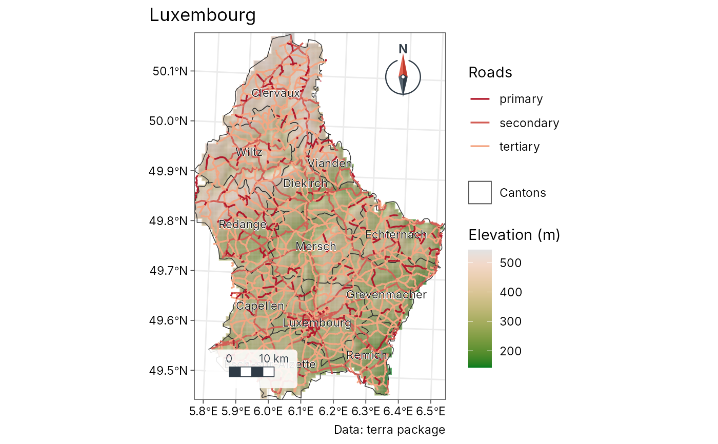
# Luxembourg: elevation, cantons, highways and canton names
# (data shipped with terra)
elev <- terra::rast(system.file("ex/elev.tif", package = "terra"))
cantons <- sf::st_read(system.file("ex/lux.shp", package = "terra"), quiet = TRUE)
roads <- sf::st_as_sf(terra::unwrap(
  readRDS(system.file("ex/lux_highways.rds", package = "terra"))
))

# \donttest{
geo_map(title = "Luxembourg", caption = "Data: terra package") |>
  map_raster(elev, name = "Elevation (m)", palette = "Terrain 2",
    hillshade = TRUE) |>
  map_polygons(cantons, fill = NA, border = "grey20", label = "Cantons") |>
  map_lines(roads, colour = highway, palette = c("#B2182B", "#F4A582"),
    group = "Roads") |>
  map_labels(cantons, text = NAME_2)

# }

Layered maps, built one layer at a time

Usage

Arguments

Value

See also

Examples