Map projections and graticules — map-projection • tidymapr

Choose a coordinate reference system by name and draw graticules (latitude/longitude lines), as in GeoSpaX.

geo_crs() returns an sf::st_crs() object for a named projection, centred on your data when that matters.
coord_projection() draws any ggplot map (including every tidymapr map) in that projection: add it with +.
map_graticule() sets the graticule interval and style, and can draw the outline of the globe on world maps.

`projection`	Use	CRS
`"equal_earth"`	World maps with true areas (recommended for world choropleths)	EPSG:8857
`"mercator"`	World Mercator: conformal, areas grow towards the poles	EPSG:3395
`"web_mercator"`	Matches online tiles (OpenStreetMap, Esri)	EPSG:3857
`"robinson"`	Compromise world map	ESRI:54030
`"mollweide"`	Equal-area world map, elliptical	ESRI:54009
`"winkel_tripel"`	Compromise world map (National Geographic)	`+proj=wintri`
`"lonlat"`	Plain longitude/latitude (WGS 84)	EPSG:4326
`"utm"`	Local maps in metres; UTM zone picked from `data`	EPSG:326xx/327xx
`"laea"`	Equal-area, centred on `data` (continents, regions)	Lambert azimuthal
`"albers"`	Equal-area conic for mid-latitude regions	Albers
`"orthographic"`	The globe seen from space, centred on `data`	orthographic

Any EPSG code (for example 32755) or PROJ/WKT string also works. World projections accept lon0 to centre the map elsewhere, for example lon0 = 150 for a Pacific-centred map that keeps Papua New Guinea in the middle; use sf::st_break_antimeridian() on world polygons first so countries crossing the new edge are split cleanly.

Usage

geo_crs(projection = "equal_earth", data = NULL, lon0 = NULL, lat0 = NULL)

coord_projection(
  projection = "equal_earth",
  data = NULL,
  lon0 = NULL,
  lat0 = NULL,
  expand = FALSE,
  ...
)

map_graticule(
  interval = 30,
  labels = "auto",
  colour = "grey80",
  linewidth = 0.25,
  linetype = "solid",
  outline = FALSE
)

Arguments

projection: Projection name (see table), an EPSG number or a CRS string.
data: Optional sf object or bbox used to centre "utm", "laea", "albers" and "orthographic".
lon0, lat0: Central longitude and latitude. Default: the centre of data, or 0.
expand: Expand the plot limits a little beyond the data?
...: Passed to ggplot2::coord_sf() (for example xlim, ylim).
interval: Graticule spacing in degrees: one number for both, or c(longitude, latitude).
labels: Which graticule lines to label: "auto" (latitudes only on curved world projections, where longitude labels would crowd the pole line; both elsewhere), "both", "latitude", "longitude" or "none". TRUE and FALSE mean "auto" and "none".
colour, linewidth, linetype: Graticule line style.
outline: Draw the edge of the map: the outline of the world on world projections, or the horizon circle on "orthographic" maps.

Value

geo_crs(): a crs object. coord_projection() and map_graticule(): settings to add to a ggplot with + (add map_graticule() after coord_projection()).

References

Šavrič, B., Patterson, T. and Jenny, B. (2019). The Equal Earth map projection. International Journal of Geographical Information Science, 33, 454-465. doi:10.1080/13658816.2018.1504949

Examples

library(ggplot2)
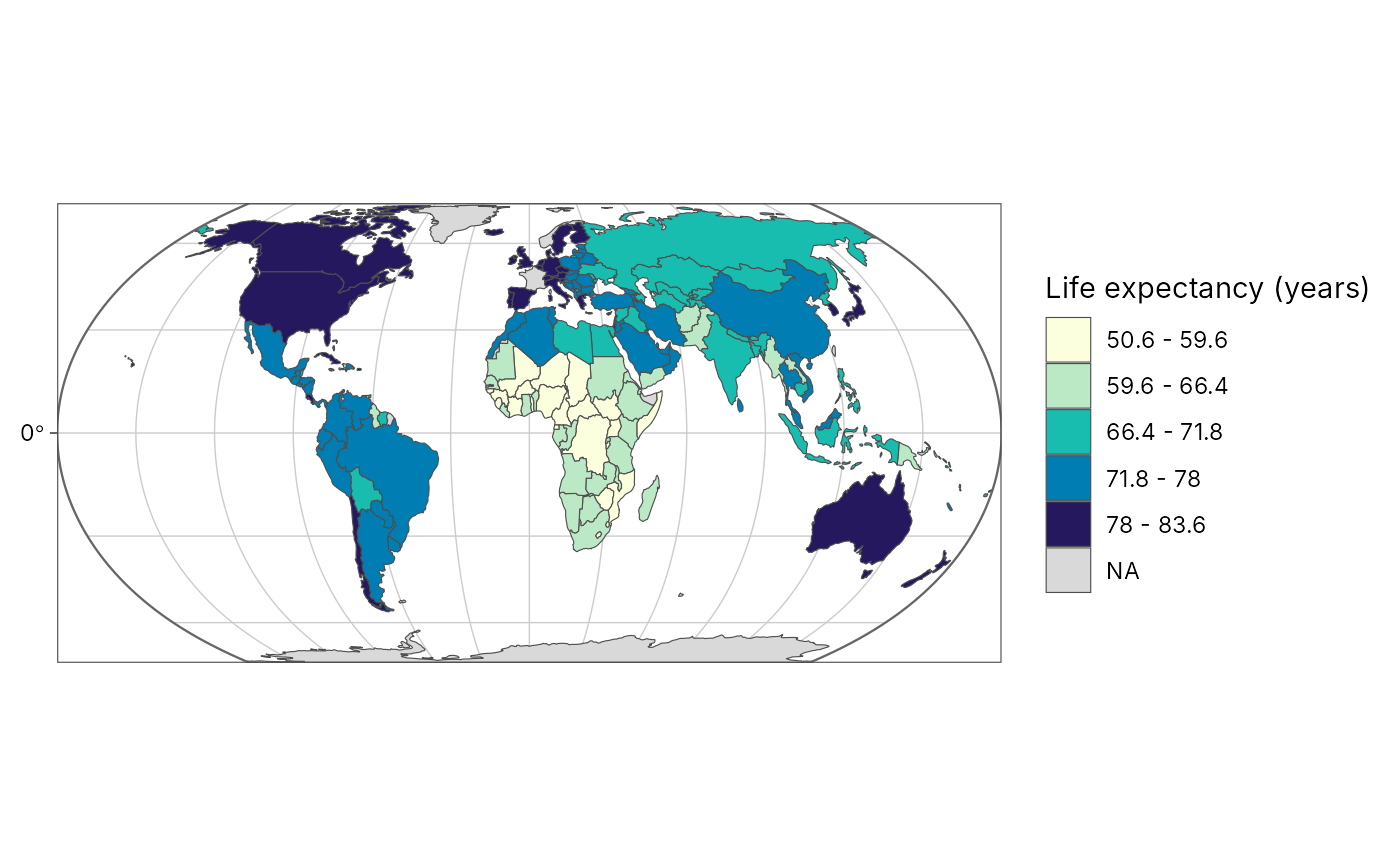
# Life expectancy by country (spData::world, Natural Earth and World Bank)
world <- spData::world
plot_choropleth(world, lifeExp, n = 5, style = "jenks",
  legend_title = "Life expectancy (years)") +
  coord_projection("equal_earth") +
  map_graticule(interval = 30, outline = TRUE)


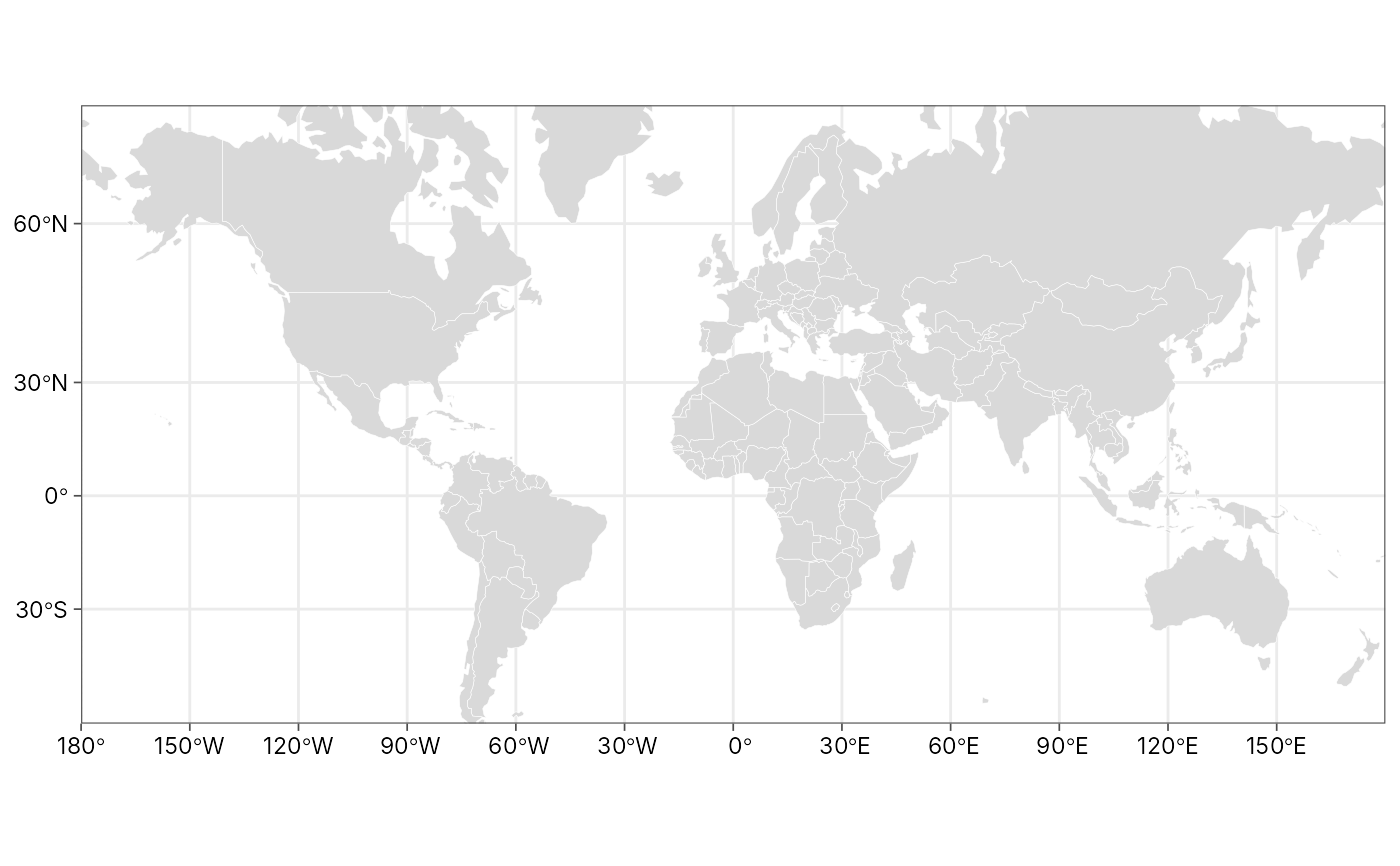
# The same world in Mercator: note how Greenland and Antarctica swell
ggplot(world) +
  geom_sf(fill = "grey85", colour = "white", linewidth = 0.1) +
  coord_projection("mercator", ylim = c(-7e6, 1.2e7)) +
  map_graticule(interval = 30) +
  theme_tidymapr()


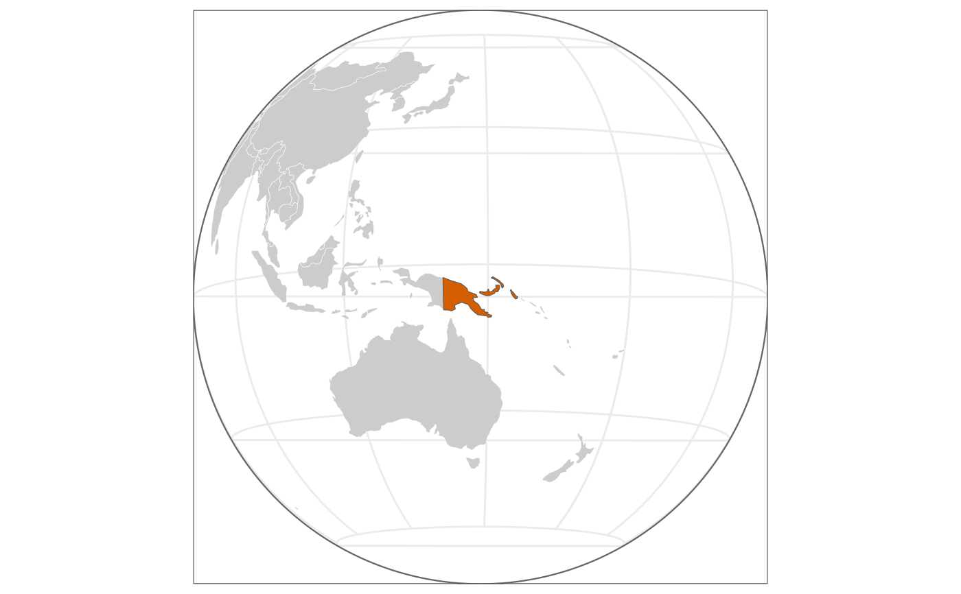
# The globe from space, centred on Papua New Guinea
png <- world[world$name_long == "Papua New Guinea", ]
ggplot(world) +
  geom_sf(fill = "grey80", colour = "white", linewidth = 0.1) +
  geom_sf(data = png, fill = "#D55E00") +
  coord_projection("orthographic", data = png) +
  map_graticule(30, outline = TRUE) +
  theme_tidymapr(grid = "none")


# Local maps: UTM zone picked from the Mt Wilhelm sites (55S)
sites <- geo_as_sf(geo_example_sites(), lon, lat)
geo_crs("utm", data = sites)$input
#> [1] "EPSG:32755"