Choropleth and bubble maps

Two classic thematic maps, drawn with ggplot2 and theme_tidymapr():

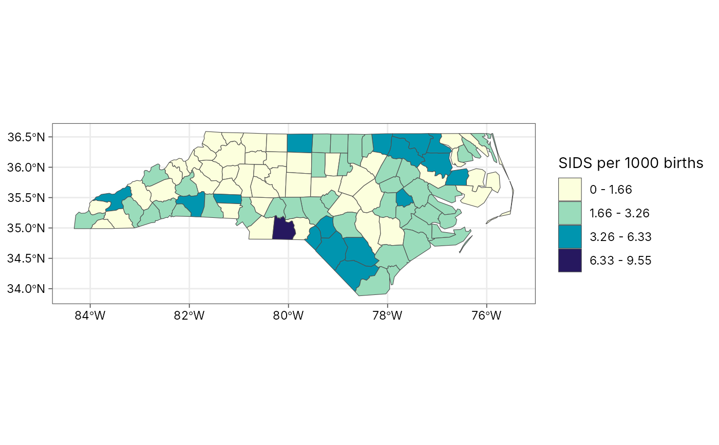
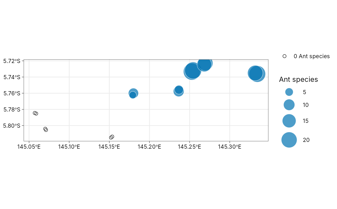
• plot_choropleth() shades polygons (regions, plots, provinces) by a numeric column. Values are grouped into classes with geo_classify() (quantile, equal, Fisher-Jenks, pretty, standard deviation or fixed breaks), so the legend shows readable ranges such as "10 - 20". The classification (breaks, counts per class and goodness of variance fit) is kept in attribute "classification" of the plot.

• plot_bubble() draws a circle at each site with its area proportional to a numeric column, the standard way to map counts such as species richness or abundance. Larger circles are drawn first, so small ones stay visible on top. Sites with a value of zero (sampled, but nothing found) are shown as small open circles, so absences stay on the map instead of disappearing.

Both return an ordinary ggplot, so you can add layers, change scales or save with geo_save().

Usage

plot_choropleth(
  data,
  value,
  n = 5,
  style = c("quantile", "equal", "jenks", "pretty", "sd", "fixed"),
  breaks = NULL,
  digits = 3,
  palette = "YlGnBu",
  reverse = TRUE,
  border = "grey30",
  linewidth = 0.2,
  na_fill = "grey85",
  legend_title = NULL
)

plot_bubble(
  data,
  size,
  lon = lon,
  lat = lat,
  colour = NULL,
  fill = "#0072B2",
  max_size = 12,
  alpha = 0.7,
  background = NULL,
  legend_title = NULL
)

Arguments

data

For plot_choropleth(), an sf table of polygons. For plot_bubble(), an sf point table or a data frame with longitude and latitude columns.

value

<data-masking> Numeric column that sets the fill class (plot_choropleth()).

n, style, breaks, digits

Classification, passed to geo_classify().

palette

For plot_choropleth(), the name of a sequential palette from grDevices::hcl.colors() (default "YlGnBu", colour-blind safe and readable in greyscale).

reverse

Reverse the palette? The default (TRUE) runs from light (low values) to dark (high values).

border, linewidth

Polygon outline colour and width.

na_fill

Fill for polygons with a missing value.

legend_title

Legend title; defaults to the column name.

size

<data-masking> Numeric column that sets bubble area (plot_bubble()).

lon, lat

<data-masking> Coordinate columns when data is not sf (plot_bubble()).

colour

<data-masking> Optional column that colours the bubbles by group (Okabe-Ito palette).

fill

Bubble colour when colour is not given.

max_size

Diameter (in points) of the largest bubble.

alpha

Bubble transparency.

background

Optional sf layer (for example a coastline or province boundaries) drawn in light grey under the bubbles.

Value

A ggplot object.

See also

geo_classify() for the classes alone; plot_sites() for study-site maps with basemaps.

Examples

# Choropleth: sudden infant deaths 1974-78 in North Carolina counties
# (real data shipped with sf)
nc <- sf::st_read(system.file("shape/nc.shp", package = "sf"), quiet = TRUE)
nc$sids_rate <- 1000 * nc$SID74 / nc$BIR74
p <- plot_choropleth(nc, sids_rate, n = 5, style = "jenks",
  legend_title = "SIDS per 1000 births")
p

attr(p, "classification")$gvf
#> [1] 0.8824022

# Bubble map: ant species observed on each Mt Wilhelm transect
# (Mottl, Moses and Klimes 2023)
# \donttest{
if (requireNamespace("tidydiversity", quietly = TRUE)) {
  richness <- tidydiversity::png_ants |>
    dplyr::distinct(site, transect, species) |>
    dplyr::count(site, transect, name = "species")
  # Transects above 2,200 m were baited but no ants came: richness 0
  sites <- png_ants_sites |>
    dplyr::left_join(richness, by = c("site", "transect")) |>
    dplyr::mutate(species = dplyr::coalesce(species, 0L))
  plot_bubble(sites, species, legend_title = "Ant species")
}

# }