Automatic publication maps that explain their choices

geo_automap() draws a finished map from one call, in the spirit of GeoSpaX's AutoMap. It looks at your data and chooses, with a reason for each choice:

projection: Equal Earth for world-wide data (true areas), a Lambert azimuthal equal-area projection centred on the data for continents and large regions, and the local UTM zone for study areas (distances in metres);
symbology, following the conventions of GeoSpaX's AutoMap, ArcGIS and QGIS:
- numbers on points, lines or polygons get graduated colours in classes (a classed legend, never a continuous ramp). The method follows the shape of the data: equal intervals when roughly symmetric (|skew| < 0.5), natural breaks (Jenks) when skewed, and quantiles when heavy-tailed (|skew| >= 2); 5 classes for 30 or more features, fewer for small samples;
- the colour ramp follows the field's meaning: blues for water and rain, greens for vegetation, viridis for elevation, slope and predictions, a diverging ramp when values cross zero, and yellow-orange-red otherwise;
- small whole-number counts on points get proportional circles;
- categories get qualitative Okabe-Ito colours; features without a value get a single symbol;
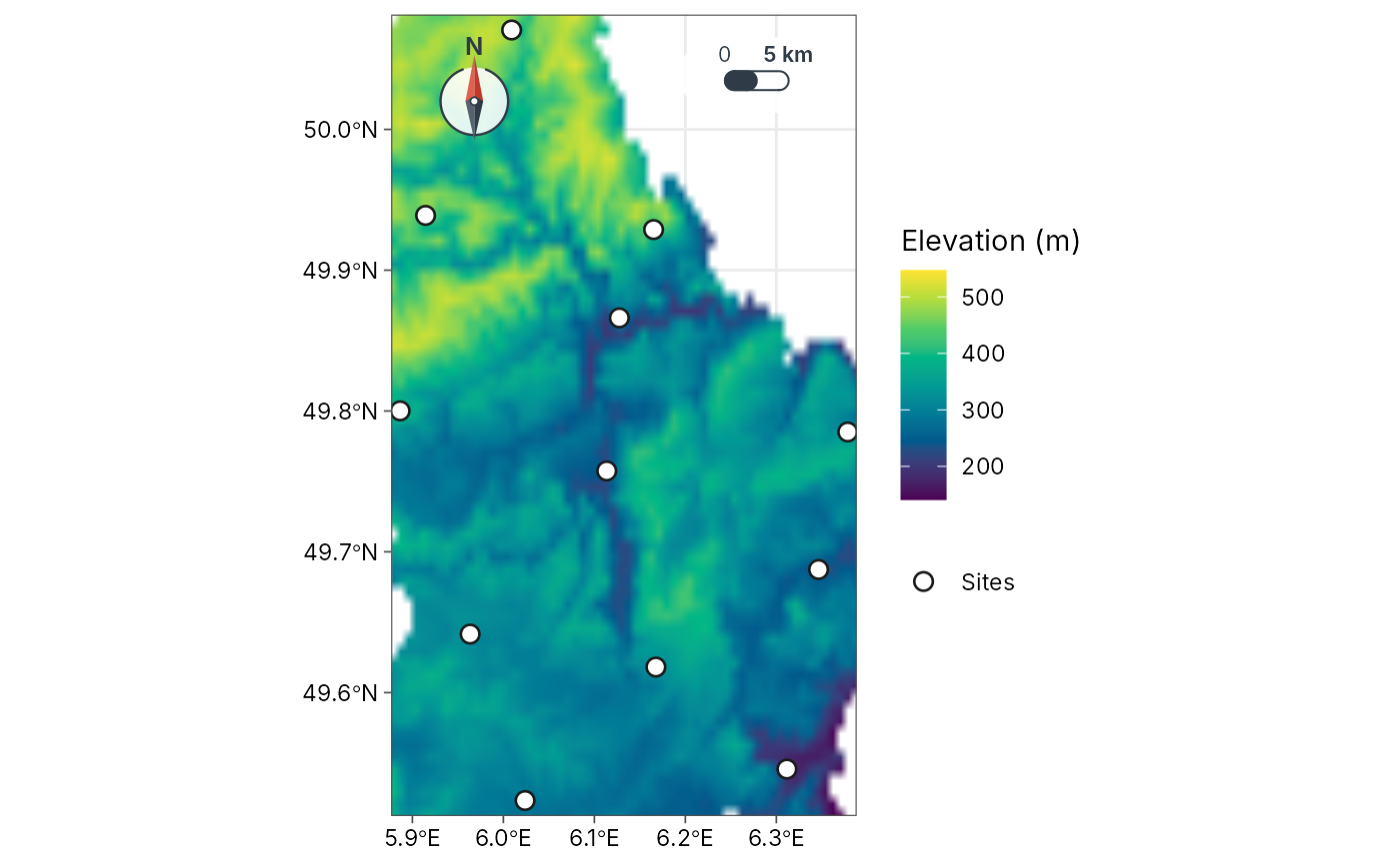
- continuous surfaces (a raster x, or a background such as a DEM under your sites) get a stretched colour ramp with a gradient legend, the only place a gradient legend is used;
basemap: none for world and regional maps or under a background surface; topographic tiles for study areas, as muted context that is not in the legend (the coastline when offline);
furniture: graticule and world outline on world maps; scale bar and north arrow on regional and local maps, in corners chosen to avoid the data.

Everything can be overridden through the arguments, and the result is a normal ggplot you can keep editing. geo_automap_explain() returns the decisions as a table, ready for a methods section.

Usage

geo_automap(
  x,
  value = NULL,
  projection = "auto",
  style = "auto",
  n = "auto",
  basemap = "auto",
  background = NULL,
  background_title = NULL,
  palette = "auto",
  background_palette = "auto",
  title = NULL,
  legend_title = NULL,
  scale_bar = "auto",
  north_arrow = "auto"
)

geo_automap_explain(map)

Arguments

x: An sf table (points, lines or polygons) or a SpatRaster.
value: <data-masking> Column to map. Omit to map the features alone (or the first raster layer).
projection: "auto" or any name accepted by coord_projection().
style: "auto" or a geo_classify() style for graduated colours.
n: Number of classes, or "auto" (5 for 30 or more features, fewer for small samples).
basemap: "auto" or a basemap name for geo_basemap().
background: Optional continuous surface (SpatRaster or file path), for example a DEM or a rainfall layer, drawn under the features with a gradient legend. With a background, the features are shown as sites (single symbol, or classes when value is given) and no tile basemap is added.
background_title: Legend title for the background.
palette, background_palette: Colour ramp for the features and for the background surface: "auto" (chosen from the field's meaning), any palette name from grDevices::hcl.pals() (for example "viridis", "Blues 3", "YlOrRd", "Terrain 2", "RdYlBu"), or a vector of colours. For categories, a vector of colours replaces the Okabe-Ito colours.
title, legend_title: Map and legend titles.
scale_bar, north_arrow: "auto", FALSE, or a style name (see annotation_scale_bar()).
map: A map from geo_automap().

Value

A ggplot with attribute "automap", the table of decisions.

Examples

# World: life expectancy by country (spData::world)
library(sf)
#> Linking to GEOS 3.12.1, GDAL 3.8.4, PROJ 9.4.0; sf_use_s2() is TRUE
m <- geo_automap(spData::world, lifeExp, legend_title = "Life expectancy")
m

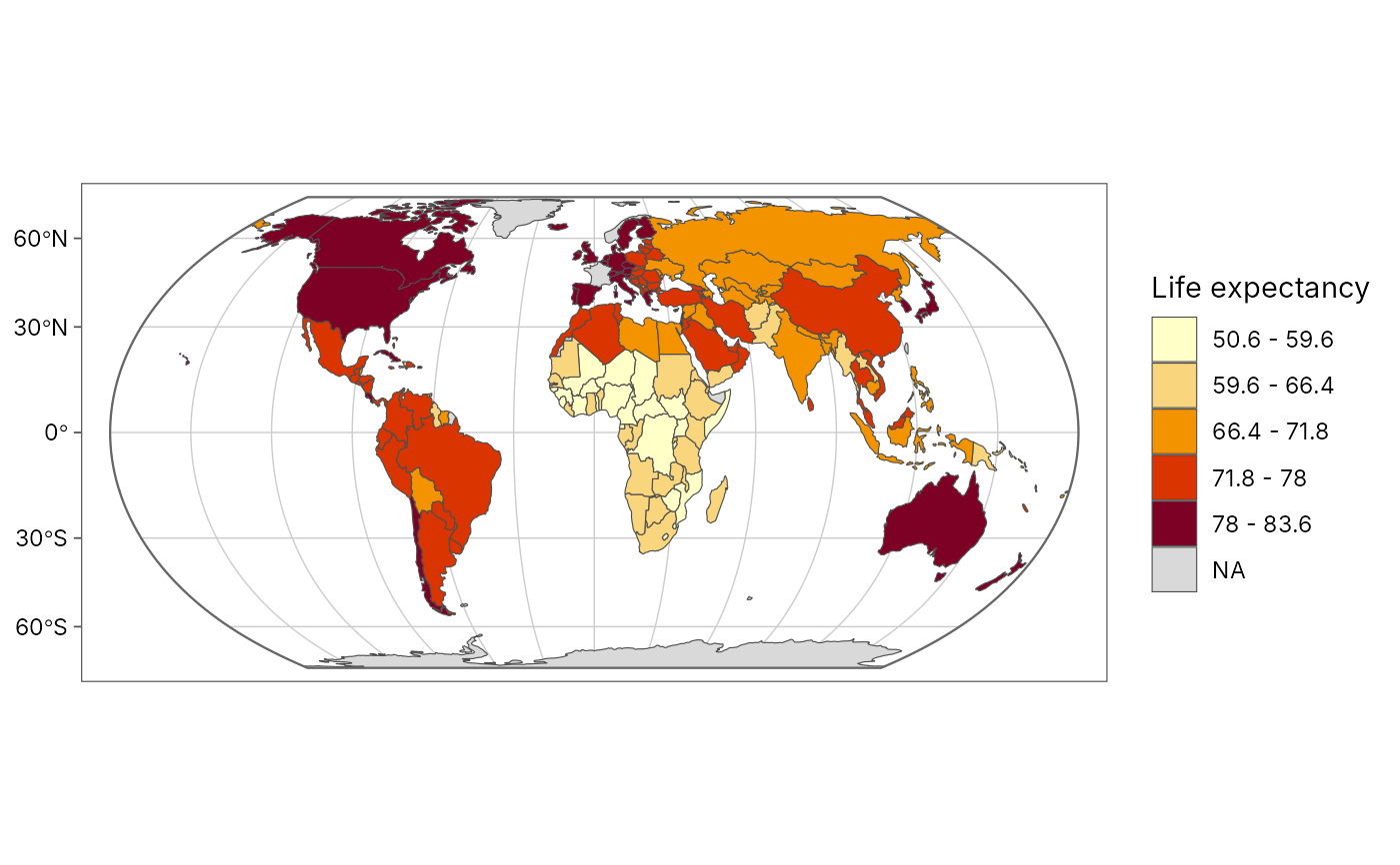geo_automap_explain(m)
#> # A tibble: 5 × 3
#>   element    choice                                       reason                
#>   <chr>      <chr>                                        <chr>                 
#> 1 projection equal_earth                                  Data span 360 degrees…
#> 2 symbology  graduated colours (jenks, 5 classes, YlOrRd) 'lifeExp' is numeric …
#> 3 basemap    none                                         Polygons, rasters and…
#> 4 graticule  30 degrees, world outline                    World map: graticule …
#> 5 scale bar  none                                         Scale varies across a…

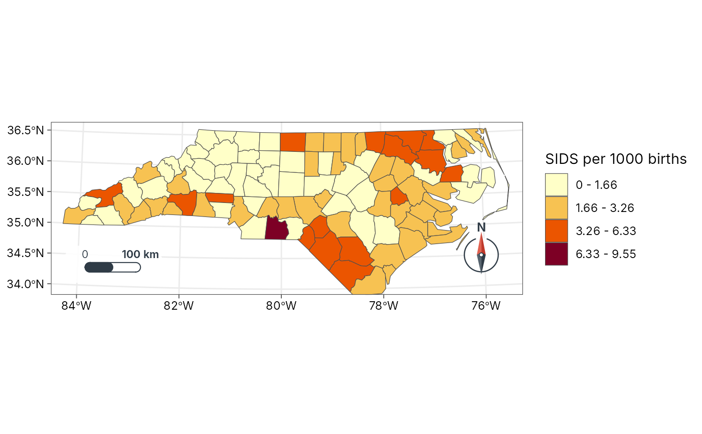
# Region: North Carolina SIDS rate 1974-78 (shipped with sf)
nc <- st_read(system.file("shape/nc.shp", package = "sf"), quiet = TRUE)
nc$sids_rate <- 1000 * nc$SID74 / nc$BIR74
geo_automap(nc, sids_rate, legend_title = "SIDS per 1000 births")


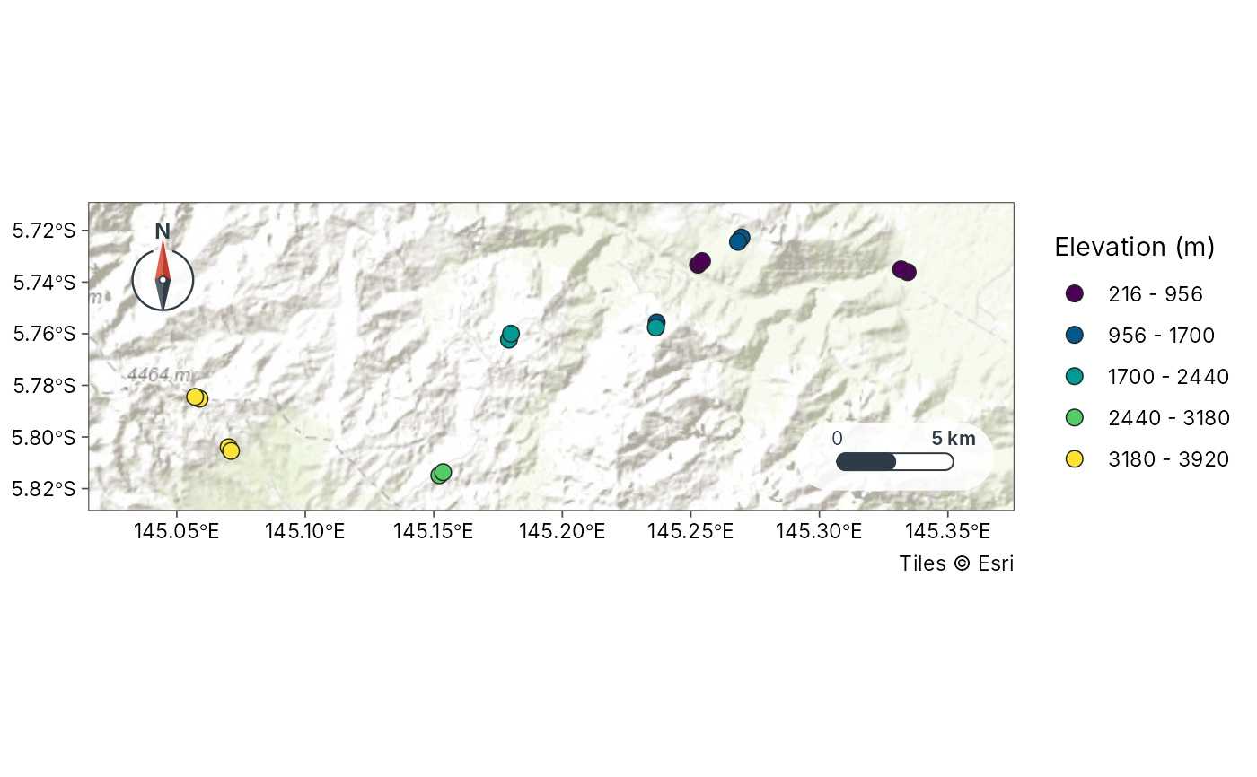
# Study area: the 16 Mt Wilhelm ant transects, classed by elevation
sites <- geo_as_sf(png_ants_sites, lon, lat)
geo_automap(sites, elevation, legend_title = "Elevation (m)")


# Choose your own ramps: an hcl palette name or any colours
geo_automap(nc, sids_rate, palette = "Purples 3")

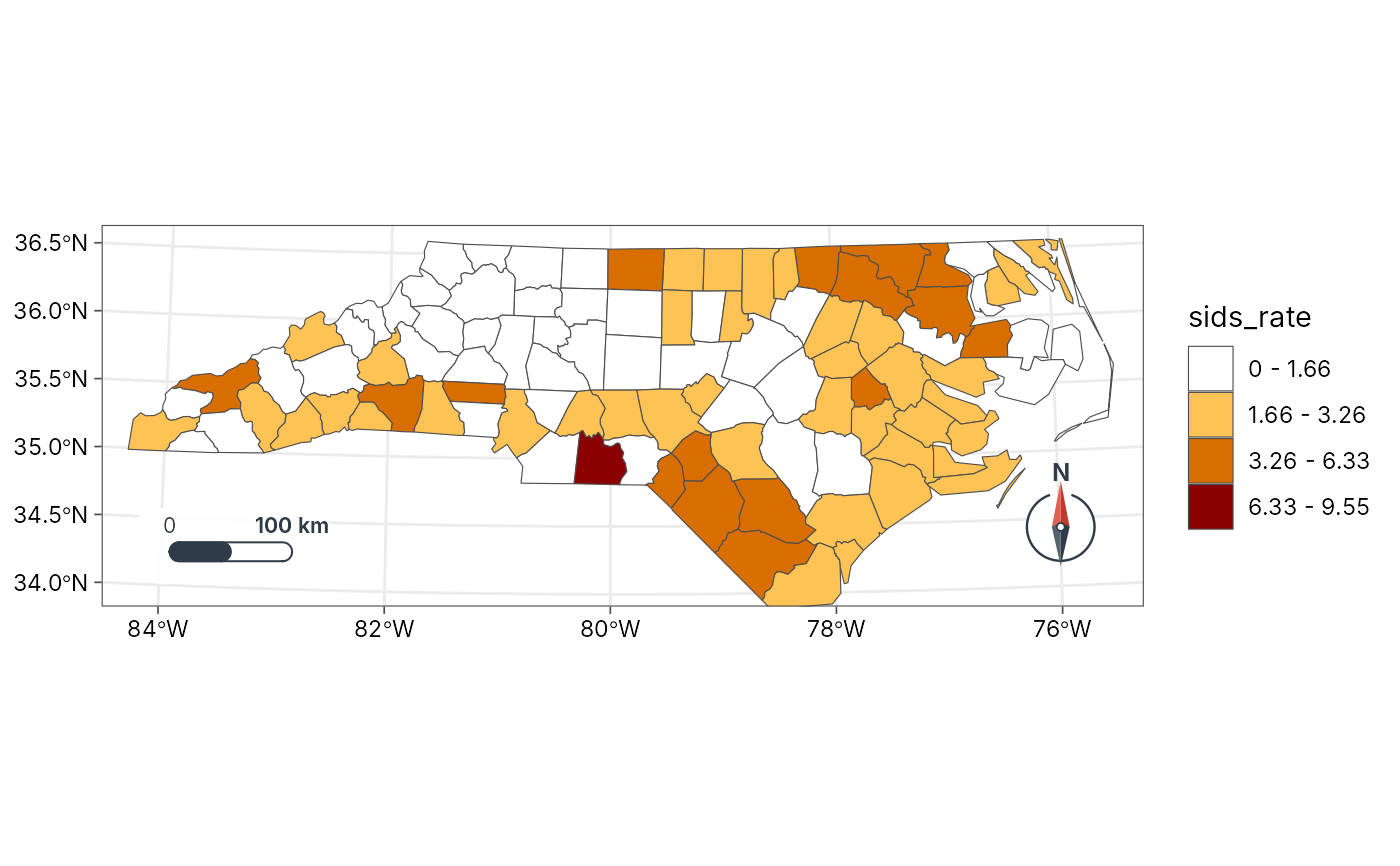
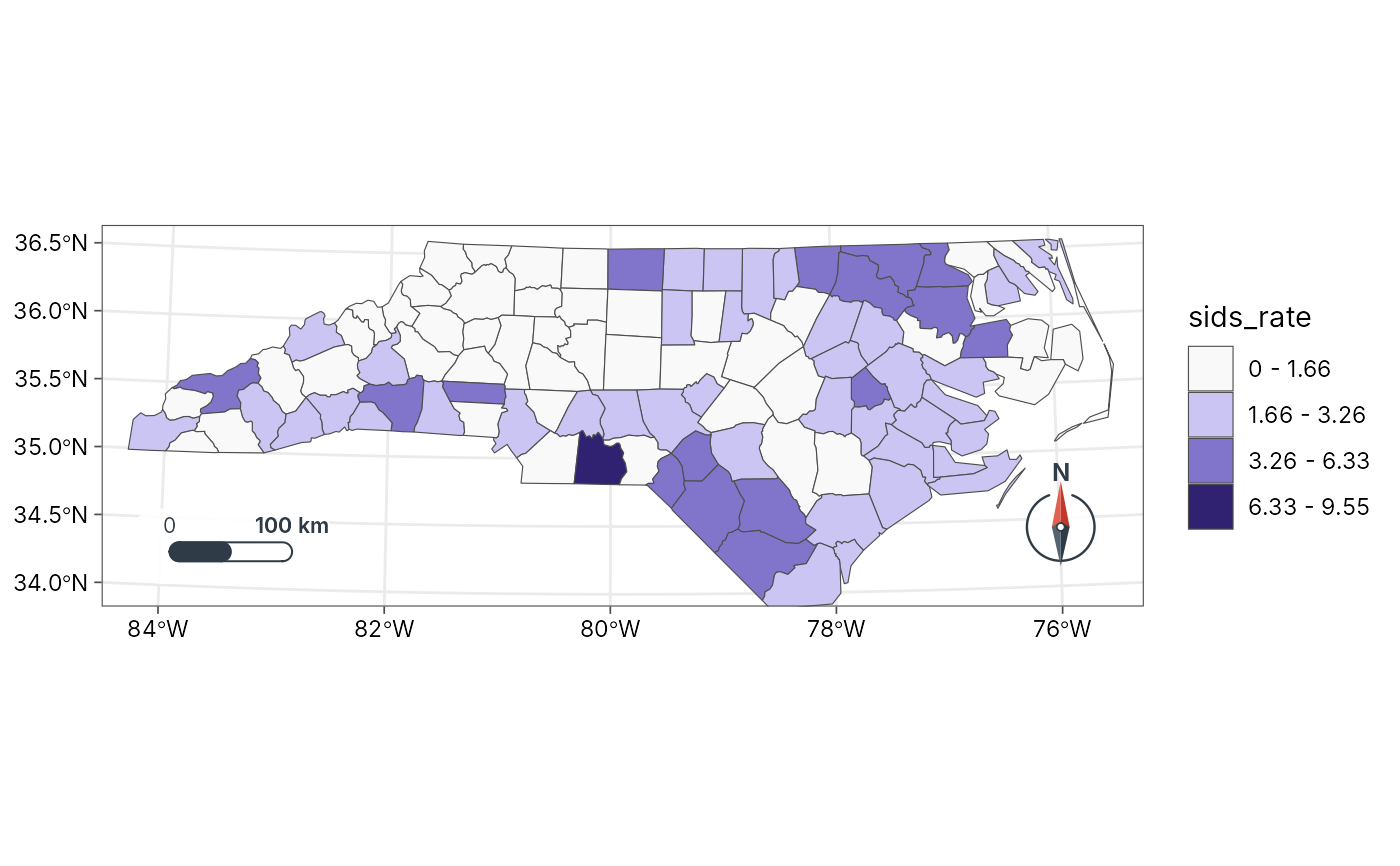geo_automap(nc, sids_rate, palette = c("white", "orange", "darkred"))


# Sites over a continuous surface: the surface gets the gradient legend
# (here Luxembourg's elevation, shipped with terra, under its cantons)
if (rlang::is_installed("terra")) {
  dem <- terra::rast(system.file("ex/elev.tif", package = "terra"))
  lux <- st_read(system.file("ex/lux.shp", package = "terra"), quiet = TRUE)
  towns <- suppressWarnings(st_centroid(lux))
  geo_automap(towns, background = dem, background_title = "Elevation (m)")
}

Automatic publication maps that explain their choices

Usage

Arguments

Value

See also

Examples